Table of Contents
EMSCOPE User’s Manual
1. General Information
1.1 Documentation
Enclosed with this manual are:
- a service questionnaire to send back to EMZER in case an equipment service is needed (see Return for Repair form at the end).
- an accessories checklist to verify all accessories enclosed in the packaging.
1.2 Introduction to EMSCOPE

Figure 1. EMSCOPE picture.
EMSCOPE is an EMZER’s instrument for ElectroMagnetic Interference (EMI) measurements that combines a 2-channel EMI-Test Receiver with a 16-A single-phase dual-port V-network Line Impedance Stabilization Network (LISN) and two Transient Limiters (one for each channel of the EMI receiver). EMSCOPE has been optimally designed and manufactured to be compliant to CISPR 16-1-1, CISPR 16-1-2 and MIL-STD-461E International Standards for measurements of conducted electromagnetic interference from 9 kHz up to 110 MHz.
EMSCOPE integrates the peak, quasi-peak and average detectors compliant to CISPR 16-1-1, which can be run in parallel and real time, considerably reducing the measurement time when compared to any other option. Additionally, it is possible to simultaneously measure the line and neutral emissions, or the common-mode and differential-mode (modal) emissions with the three detectors running simultaneously. Modal-emission measurements are fundamental to know the dominant mode and to implement the suitable power-line filter accordingly, using fewer components and getting a cheaper design.
EMSCOPE can be connected to a LAN or reached by direct connection (using the supplied optical fibre), and it is remotely controlled using any standard web browser, without the necessity of any additional software. The web-based application installed in EMSCOPE exhibits a very friendly and intuitive interface that makes any kind of measurement really easy to be configured.
Important! Before using the LISN, all safety requirements must be fulfilled.
1.3 Instrument Items
EMSCOPE includes the following items:
- EMSCOPE enclosure containing two EMI-Test Receivers, a 16-A single-phase dual-port V-network LISN and two Transient Limiters.
- TP-Link multimode fibre to Ethernet converter.
- IEC C20 cable.
- IEC C14 cable.
- SFP multimode optical fibre 50 or 62.5/125 µm, LC-LC connectors (1000BASE-SX standard). Wavelength: 850 nm.
- Operating Manual.
- Certificate of Calibration.
- Return for Repair form.
1.4 Optional accessories
Additionally to the multi-mode fiber to Ethernet converter, EMZER can supply a multi-mode fiber to USB converter to directly connect the computer to the EMSCOPE. The model supplied is:
- DIGITUS USB 3.0 Gigabit SFP Network Adapter (Digitus DN-3026) with a fibre optic transceiver (Digitus DN-81000).
Important! It is highly recommended to use this option with a USB-3.0 port.
1.5 Other accessories
EMSCOPE can be used with:
- External LISNs of any type
- Near Field Probes
- Current probes
1.6 Main Specifications
Table 1-1 lists the main specifications of the EMI receiver and the LISN, and Table 1-2 those of the oscilloscope mode.
| Table 1-1 Main Specifications of the EMI Receiver | |
|---|---|
| Electrical Characteristic | Performance Limits |
| Frequency range / RBW Filter Resolution / RBW Filter Frequency accuracy | 9 kHz to 150 kHz / 200 Hz 9 kHz to 150 kHz / 1 kHz 150 kHz to 30 MHz / 9 kHz 150 kHz to 30 MHz / 10 kHz 30 MHz to 110 MHz / 120kHz 113 Hz / 200Hz 509 Hz / 1kHz 5087 Hz / 9kHz 5087 Hz / 10kHz 30.52 kHz / 120kHz ≤ 2.5 ppm @ operating temperature range = 1.5 ppm @ 25 °C |
| RF inputs VSWR Attenuator Transient limiter | ZIN 50 Ω, N fem. < 1.2 0 dB to 78 dB (1 dB step) Built in up to 30 MHz. 1dB compression point: 23dBm |
| Max input level (without equipment damage) | 144 dBμV (5W, 37 dBm) |
| Noise level (Att. 22 dB, 50 Ω term., Hold Time 1 s) 9kHz to 150kHz (200Hz RBW) 9kHz to 150kHz (1kHz RBW) 150kHz to 30MHz (9kHz RBW) 150kHz to 30MHz (10kHz RBW) 30MHz to 110MHz (120kHz RBW) | < -9 dBμV (QP) < -15 dBμV (AV) Not defined (QP) < -13 dBμV (AV) < 7 dBμV (QP) < 0 dBμV (AV) Not defined (QP) 3 dBμV (AV) < 27 dBμV (QP) < 15 dBμV (AV) |
| Detectors | Peak, Quasi-peak, CISPR Average (all can be run simultaneously on both lines, that is, up to 6 detectors) |
| Type of measurements | Physical (or circuit, i.e. line and neutral) and modal (common and differential mode) conducted emissions |
| Full spectrum measurement time | Equal to the measurement dwell time, which is totally configurable from 1s to 15s |
| Display units | dBm, dBmV, dBµV, Watts, Volts |
| Measurement accuracy for sinusoidal signals > 20 dB | 9 kHz to 150 kHz / 200 Hz ± 1.5 dB 9 kHz to 150 kHz / 1 kHz ± 1.5 dB 150 kHz to 30 MHz / 9 kHz ± 1.5 dB 150 kHz to 30 MHz / 10 kHz ± 1.5 dB 30 MHz to 110 MHz / 120 kHz ± 1.5 dB |
| CISPR 16-1-1 conformity | Standard compliant QP detector down to 1 Hz PRF for bands A and B. Down to 10 Hz PRF for band C. Standard compliant Average detector down to 1 Hz PRF for bands A and B. Down to 10 Hz PRF for band C. |
| I/O Interface | SFP Optical |
| Operating temperature | 0 °C to 40 °C |
| Power supply | 100-240 VAC, 50/60 Hz. Consumption: 25 W max |
| Dimensions (W x H x D) | 252 x 195 x 438 mm |
| Weight | 8.5 kg |
| Built in LISN | Fully compliant to CISPR 16-1-2 standard |
| Frequency range | 9 kHz to 30 MHz |
| Continuous rated output current | Up to 16 A @ 230 VAC (socket dependent)* |
| Max permissible operating voltage | Up to 300 VAC – 325 VDC (socket dependent)* |
| EUT supply frequency range | DC to 60 Hz |
| CISPR equivalent circuit / Pre-filter Choke | 50 Ω / / (50 μH + 5 Ω) / 250 μH |
| EUT Power connector / mains | Schuko socket (Type F) / IEC C20 |
| Artificial Hand / connector type | 510 Ω + 220 pF / 4 mm socket |
* Socket dependent. Examples of sockets:
- NEMA 5-15R: 15A / 125Vac
- EU Type F: 16A / 230Vac
- GB BS1363 Type G: 13A / 250Vac
Notes:
- The LISN and all of its components can handle 300V, 16 amps.
- Full compliance with CISPR 16-1-1 has been achieved by accrediting the detectors using the pulsed-tone method in an accredited laboratory. Any customer wishing to accredit the receiver down to 1 Hz must do so in an EMC laboratory that follows this same method.
| Table 1-2 Main Specifications of the Oscilloscope Mode | |
|---|---|
| Characteristic | Performance |
| Channels | 2 (Line and Neutral, or CM and DM) 4 on three-phase models (L1, L2, L3 and N, or CM, DM1, DM2 and DM3), all sampled simultaneously |
| Bandwidth | 9 kHz to 110 MHz (AC coupled: no DC component is shown) |
| Resolution | 16 bits |
| Sampling frequency | Up to 250 Msps per channel (Table 5-1) |
| Memory depth | 8k to 10M samples per channel |
| Time division factor | 1 µs/div to 200 ms/div (with zoom down to the individual samples) |
| Amplitude division factor | 1 mV/div to 5 V/div per channel, at the receiver input |
| Acquisition | Normal, Peak detect, Hi-res; Average (2 to 1024 captures) and Envelope across captures |
| Trigger | Edge, Pulse width, Window and Burst on any channel at the full 250 Msps (4 ns resolution); Normal / Auto modes, adjustable or automatic hysteresis, HF reject (5 MHz, 620 kHz, 78 kHz) |
| Automatic measurements | 16 voltage, time and between-trace measurements (phase, delay), with statistics |
| Math | A + B, A − B, A × B |
| Capture export | CSV (up to 1M samples) and binary (up to 10M samples, with readers for Python and MATLAB) |
1.7 Front Panel
The front panel of the EMSCOPE is shown in the next figure.

Figure 2. Front panel.
Connectors and indicators of the front panel from top to bottom:
- LEDs
- RF input 50 Ω connectors
The equipment has 2 N female RF input 50 Ω connectors that allow the equipment to simultaneously measure 2 RF signals. Each RF input is internally protected from transient voltages by means of a transient limiter. The technical characteristics are described in the Main Specifications section.
- RF output connectors
The equipment has 2 N female RF output connectors. Each connector is the output of a channel of the artificial mains network (LISN). These connectors output the conducted interferences generated by the equipment under test and provide the means to measure them.
- Output mains power network supply socket
This socket is the output of the artificial mains power network of the LISN. It is the mains socket where the equipment under test must be connected to allow the measurement of its conducted emissions. The technical specifications of the LISN and its power handling capabilities are described under the Main specifications section.
- Artificial Hand 4mm socket
This socket provides the RC network required to mimic the behaviour of a hand for a handheld equipment under test, as stated in the CISPR 16-1-2. This RC network is described in the Main Specifications section.
- Protective earth terminal. It is a M6 threaded bolt for connecting the protective earth conductor.
- Additionally, there exist two 4mm female sockets for connecting the reference ground during calibration.
1.8 Rear Panel
The rear panel of the equipment is shown in the next figure:

Figure 3. Rear panel.
Connectors of the rear panel from top to bottom:
- SFP connector. The installed SFP transceiver is described in the Instruments Items section.
- Instrument power supply socket. It includes fuses and the On-Off switch.
- IEC-20 socket. It is the socket of the mains power supply that cross the LISN and feeds device under test.
- Grounding bar. This bar provides an appropriate RF ground reference and it should be connected to the grounded RF plane as described in different standards (e.g. CISPR 16-2-1).
- Additionally, there exist two 4mm female sockets for connecting the reference ground during calibration.
1.9 EMSCOPE Overview
The EMSCOPE features a completely new receiver architecture based on the most recent FPGA technology that includes a two port CISPR 16-1-2 LISN and two 10-dB transient limiters, and has been designed to be controlled using only a web browser, independently of the operating system and platform. No additional software is required.
In the CISPR bands A (9 kHz ÷ 150 kHz), B (150 kHz ÷ 30 MHz) and C (30 MHz ÷ 110 MHz) the standards require the use of specially shaped 200-Hz, 9-kHz and 120-kHz filters respectively (1-kHz and 10-kHz filters in the MIL-standard case). EMSCOPE makes use of internal numerically modelled filters in compliance with the norms, using FFT and signal processing techniques, which allows to perform measurements according to both standards (CISPR and MIL). Besides, it can provide simultaneous and real-time measurement results using the peak, quasi-peak and average detectors in compliance with CISPR 16-1-1.
The CISPR 16-1-2 compliant LISN integrated in the instrument allows performing conducted-emission measurements without any other device, making EMSCOPE a complete measurement setup. Additionally, it can also be easily connected to other external LISNs, using its external N connectors, to perform EMI measurements according to any other standard. Thanks to its architecture and to the large internal computation capability, the EMSCOPE can perform a precise entire band test in an extremely short time. This feature is not only useful to greatly increase the productivity of the test lab, but also to make better and more comprehensive analysis in case the disturbance to be evaluated is somehow intermittent and with an irregular repetition rate. Since it is possible to perform a modal analysis of the interference, providing the common-mode and differential-mode measurements, it is really easy to design a suitable power-line filter for the EUT.
Additionally, EMSCOPE incorporates an oscilloscope mode to visualize the conducted emissions in the time domain, providing more information about the connected EUT (see Oscilloscope Operating Instructions), and a clickmeter mode to evaluate discontinuous disturbances according to CISPR 14-1 (see Clickmeter Operating Instructions).
2. Safety information
2.1 General safety information
Never remove the cover or any part of the housing. During operation, there are parts with DANGEROUS voltages inside the unit.
Do not insert any objects into the openings of the housing that are not intended for that purpose. This can cause short circuits inside or electric shocks/injuries.
The unit is not protected against the penetration of liquids. Do not close any of the openings needed for ventilation.
Since the ventilation air flows from the bottom side, the unit must be placed on a non-flammable base in order to prevent a fire in case of overheating.
2.2 Safety information regarding the Line Impedance Stabilization Network (LISN)
Important! Over current protection is not provided. The LISN must be connected to a power mains which has an appropriately rated mains protection installed.
Important! Before putting into service ensure that:
- An additional PE conductor is connected (see next paragraph).
- The ventilation openings are unobstructed.
Important! Earth connection: Precautions must be taken because, since the LISN is compliant to CISPR 16, it cannot inherently adhere to the permitted leakage current limit value according to EN 61010-1 and basic insulation of a protection class I. Due to this inherent high leakage current to ground of this kind of equipment an additional protective earth connection must be supplied prior connecting the unit to the mains power supply. For this purpose, the equipment is provided with an earth grounding bar at the rear panel and additionally a protective earth screw is provided at the front.
In addition, due to this high leakage current (above 1 A), it is not possible to use a residual current operated circuit breaker. It is strongly recommended to use an isolating transformer.
During long-term operation at maximum load, the surface of the unit may exceed 60 °C.
3. Installation
3.1 Introduction
This section provides the information needed to install your EMSCOPE. It includes the information pertinent to initial inspection and power requirements, connections, operating environment, instrument mounting, cleaning, storage and shipment.
Important! Before connecting the equipment follow the provided Safety information section. Not following it can result in important damages, serious injuries and death.
3.2 Initial Inspection
When receiving the equipment, first inspect the shipping box for any damages. If the shipping box is damaged, it should be kept until the contents of the shipment have been checked for completeness and the instrument has been checked mechanically and electrically.
3.3 Packing and Unpacking
Verify the availability of all the shipped items with reference to the shipping check list enclosed with the User Manual. Notify any damage to the forwarder personnel as well as to your EMZER Representative.
To avoid further damage, do not turn on the instrument when there are signs of shipping damage to any portion of it.
3.4 Preparation for Use
The EMSCOPE EMI Receiver is a Safety Class I apparatus, and it is also equipped with protective/functional earth terminals on the rear and front panels. A good safety/functional ground connection should be provided before operating the system.
Important! The EMSCOPE LISN constructed according to the standard CISPR 16 can NOT comply with the permissible leakage current limit stated in the IEC 61010 for a class I equipment. The instructions provided in the Safety Information section must be followed.
3.5 Power Supply
The universal adapter supplied with the receiver can work at either 50 Hz or 60 Hz with a supply voltage rated between 100 and 240 Volt. When the power supply is switched ON, the leftmost green LED lights up. About 45 seconds to one minute after switching on (depending on the network), the EMSCOPE is ready for use and the rightmost LED turns green.
3.6 Front Panel LEDs
The front panel of the EMSCOPE has three LEDs, which provide some information to the user:
- The leftmost green LED is switched on when the EMSCOPE is powered on.
- The middle yellow LED blinks according to the network activity.
- The rightmost LED is fixed green and switches on when the EMSCOPE is ready to operate. It switches to purple when a user connects, and returns to green when the user disconnects.
3.7 Environment
The operating environment of the receiver is specified to be within the following limits:
- Temperature : 0 °C to +40 °C
- Humidity : < 85% relative LISN; < 95% relative EMI receivers
- Altitude : 3000 meters
The instrument should be stored and shipped in a clean, dry environment which is specified to be within the following limitations:
- Temperature : -40 °C to +50 °C (-40 °C to +40 °C for long periods)
- Humidity : < 95% relative (< 80% relative for long periods)
- Altitude : 15000 meters
3.8 Return for Service
If the instrument should be returned to EMZER for service, please complete the service questionnaire enclosed with the User Manual and attach it to the instrument.
To minimize the repair time, be as specific as possible when describing the failure. If the failure only occurs under certain conditions, explain how to duplicate the failure.
If possible, reusing of the original packaging to ship the equipment is preferable.
In case other package should be used, ensure to wrap the instrument in heavy paper or plastic.
Use a strong shipping box and use enough shock absorbing material all around the equipment to provide a firm cushion and prevent movement in the shipping box; in particular protect the front panel.
Seal the shipping box securely.
Mark the shipping box FRAGILE to encourage careful handling.
3.9 Equipment Cleaning
Use a clean, dry, non-abrasive cloth for external cleaning of the equipment.
To clean the equipment do not use any solvent, thinner, turpentine, acid, acetone or similar matter to avoid damage to external plastic or display surfaces.
3.10 Equipment Ventilation
To allow correct equipment ventilation, ensure that the vent grids on the side and on the bottom of the equipment are free by any obstructing object.
3.11 Hardware Installation
EMSCOPE is delivered from factory ready to use. After removing the instrument from its cardboard shipping box, the user must perform the following connections before switching it on:
- Connect EMSCOPE to the suitable networking technology. To this end, connect a multimode fibre from the EMSCOPE’s SFP port to the SFP port of the user’s media converter module. And then, connect the user’s media converter module to one of the following options:
- The user’s Local Area Network (LAN), using a UTP Ethernet cable. In this case, the media converter module is a Gigabit Ethernet Media Converter. An example (among others) of such converter is: tp-link MC220L.
- The remote computer (direct cable connection). In this case, the media converter module is a Fibre Optic Converter that is directly connected to the computer. An example (among others) of such converter is: US1GA30SFP from Startech.com, that directly connects to the computer’s USB port.
- Connect the instrument to the power-line network from the rear panel. Be sure to use the IEC C14 cable on the mains socket called “LINE”. The mains socket called “EUT POWER INPUT” needs an IEC C20 cable and does not supply power to the EMSCOPE.
After having done these connections, the instrument can be switched on with the Power button. The leftmost green LED lights up to indicate that the instrument is correctly powered.
The EMSCOPE then boots and runs the firmware which manages the receiver. Once the web server is ready (after about one minute), the rightmost LED turns green, informing that the receiver is ready to use (see Front Panel LEDs).
3.12 Web Connection
3.12.1 Dynamic configuration
EMSCOPE is a network attachable device focused on simple connectivity and quick accessibility, and it does not require the installation of any additional software:
- When connected to a typical LAN where there is a DHCP server (i.e., a router), EMSCOPE will automatically acquire an IP address.
- If the direct cable connection option is opted, or the LAN has no DHCP server, EMSCOPE will automatically assign itself an IP address (it uses the IPv4LL, «Dynamic Configuration of IPv4 Link-Local Addresses» -IETF RFC3927- protocol).
In either case, the user will be able to access the device by its MDNS name. To this end, open the web browser in the remote computer and type the following address in the URL field:
http://emscope-xxxx.local/
where xxxx are the last 4 characters from the SN of your EMSCOPE. The SN is provided in the rear panel. Alternatively, if known, the IP address can also be directly written in the URL field. After the last step you will get the EMSCOPE main page as shown below (please check the Troubleshooting Guide section of this document if EMSCOPE cannot be reached).

Figure 4. EMSCOPE main’s page.
3.12.2 Static Configuration
If the user wants to set the IP, it can be done in the configuration interface. To this end, click on the “Device Configuration” tab, and then “Network Configuration”. Alternatively, the same webpage is reachable by typing the following address in the URL field:
http://emscope-xxxx.local/ipconfig.php
where xxxx are the last 4 characters from the SN of your EMSCOPE. The SN is provided in the rear panel. The network configuration interface opens. By selecting the “Static IP configuration” option, an appearance similar to the interface shown in Figure 5 is obtained. The desired network configuration can be introduced following the described indications.

Figure 5. Network configuration interface.
Allowed static IP addresses are limited to class A and C.
| Table 2-1 Private IP Addresses | |||
|---|---|---|---|
| Class | Private Network | Subnet Mask | Address Range |
| A | 10.0.0.0 | 255.0.0.0 | 10.0.0.1 - 10.255.255.254 |
| C | 192.168.0.0 | 255.255.0.0 | 192.168.0.1 - 192.168.255.254 |
3.13 Using the Line Impedance Stabilization Network (LISN)
Important! Before using the EMSCOPE's built-in LISN, follow the provided Safety information. Not following it can result in important damages, serious injuries and death.
EMSCOPE must be bonded to the Protective Earth (PE) using the grounding bar placed in the rear panel. In case of using an external LISN, both need to be connected to the same PE.
To connect the EMI receivers to the built-in LISN for conducted interference measurements of an EUT, use the two N-connector bridges provided to connect the RF outputs of the LISN to the RF inputs of the receiver.
In order to avoid the unwanted tripping of the protection devices (due to the high leakage current inherently present in the LISN due to its construction made according to CISPR 16-1-2), an insulation transformer shall always be used between the mains supply and the LISN.
3.14 Transient Limiters
The built-in transient limiters are used to protect the input of the receiver from transient over voltages. Sometimes, the conducted disturbances entering the receiver through the LISN are too high - even if they cannot be seen on the EMSCOPE because they are out of the measurement bandwidth - and the associate energy is high enough to damage the input circuit. Two transient limiters (one for each line) are integrated in the system as a protection of the input from unexpected pulses and transients.
The transient limiters start clipping the input signal at 20 dBm (126.9 dBμV). The maximum input level that the transient limiters can withstand without causing equipment damage is 5 W (144 dBμV or 37 dBm), considering an input impedance of 50 Ω.
3.15 Quick start: connecting to EMSCOPE
To put EMSCOPE into operation and access it from a remote computer:
- Remove EMSCOPE from its cardboard shipping box.
- Connect a multimode fibre from the EMSCOPE SFP port to the SFP port of the media converter.
- Connect the media converter either:
- To your LAN using a UTP Ethernet cable (Gigabit Ethernet media converter, e.g. TP‑LINK MC220L), or
- Directly to the remote computer using a fibre optic converter (e.g. StarTech US1GA30SFP).
- Connect the EMSCOPE rear-panel “LINE” mains socket using the supplied IEC C14 cable. Do not use the “EUT POWER INPUT” socket to power the EMSCOPE.
- Press the Power button. The leftmost green LED turns on to indicate that the instrument is powered. After about one minute, the rightmost LED turns green when the web server is ready.
- On the remote computer, open a web browser and type http://emscope-xxxx.local/ in the address bar, where xxxx are the last four characters of the EMSCOPE serial number on the rear panel.
- If EMSCOPE cannot be reached, try using its IP address directly or refer to the “Troubleshooting Guide” section.
If the connection with the instrument is lost while the interface is open (the instrument is switched off, the network fails or the software restarts), a blue banner at the top of the page says since when there is no connection, and that it is trying to reconnect. The graphs keep the last traces, dimmed, with a small No data since stamp and the time in the bottom-right corner, so that they are not taken for a current measurement. The menu entries that need the instrument stay visible but dimmed, and do nothing when clicked (hovering shows Not available without the instrument); Save & Load still works, so what is on screen can be saved (Save measures in CSV, Save graph image). The saved image is not dimmed. When the instrument answers again, the page reloads by itself and recovers the session.
If the connection is up but the instrument stops sending measurements for longer than 15 seconds plus three dwell times (while measurements are expected: an EMI mode with a visible trace that is not frozen, outside a band change or a report), a magenta banner says The instrument is not sending measurements since …. It goes away by itself when measurements arrive again; if it stays, restart the instrument.
Only one computer can use the EMSCOPE at a time. If another computer already has the interface open, the page shows This EMSCOPE is in use from another computer and does not connect. Close the interface on the other computer, or wait until that session ends, and press Try again.
4. EMI Receiver Operating Instructions
This section introduces the instrument interface, describes some important parameters that must be known for a suitable configuration of the instrument when configured in EMI receiver mode, and explains its main utilities.

Figure 6. EMI mode.
4.1 Introduction
The EMSCOPE EMI Receiver is connected using a web browser as described above. The first time a user connects to the EMSCOPE (or when connecting using a clean session), a measurement with the default configuration is provided: one single trace measuring channel 1 (Line), RBW at 9kHz, Span 150 kHz – 30 MHz, Peak detector, Ref. Level at 115 dBμV, automatic attenuation, among other configurations.
The interface of the web app is shown in Figure 7. This interface has three important blocks. The red one contains the Main Menu, where the function keys are displayed. Each function key opens a submenu with the Action List (orange block), that is, all those settings that the user can configure for that function key. Each modification will be reflected in the Measurement Plot (blue block).

Figure 7. Web app interface.
The most relevant information regarding the measurement for each trace is provided in the trace tab, so the user can easily know what kind of measurement is currently configured. Information regarding the Center Frequency, Span and amplitude levels are reported on the top right corner.
If the user modifies the measurement configuration and closes the session, next time the user connects again to the EMSCOPE, the last configuration before closing is recovered.
Next Sections relate important considerations for the measurements and describe the relevant settings of the function keys.
4.2 Overload
For a correct measurement, be sure not to overload the EMSCOPE. Input attenuation must be properly configured considering the maximum amplitude expected at the input ports. Table 3-1 shows the maximum amplitude values that should be measured for each attenuator value to avoid distortion. If the signal surpasses this value, the EMSCOPE is saturated and will not present correct measurement values.
Important! Carefully consider that:
- Although EMSCOPE does not show any frequency bin with an amplitude value above the levels shown in Table 3-1, it may become saturated if the time-domain representation of the measured spectra is above them (saturation is produced in the ADC before processing the input signal). When this happens, a warning message is displayed in the measurement.
- Signals above 20 dBm will not be correctly measured in any case due to the activation of the transient limiters, clipping the input signal.
- Signals above 37 dBm (5 W) are not supported by the transient limiters and will damage the receivers.
- In case that an OVERLOAD indication occurs when using maximum attenuation, it is necessary to add an external attenuator to carry on the measurement without exceeding the declared limit. The user can use the “External Loss Attenuation” option to compensate the additional losses.
| Table 3-1 Maximum amplitude values | ||
|---|---|---|
| Attenuator value (dB) | Maximum Amplitude (dBm) | Maximum Amplitude (dBμV) |
| 0 | -28 | 79 |
| 1 | -27 | 80 |
| 2 | -26 | 81 |
| 3 | -25 | 82 |
| 4 | -24 | 83 |
| 5 | -23 | 84 |
| 6 | -22 | 85 |
| 7 | -21 | 86 |
| 8 | -20 | 87 |
| 9 | -19 | 88 |
| 10 | -18 | 89 |
| 11 | -17 | 90 |
| 12 | -16 | 91 |
| 13 | -15 | 92 |
| 14 | -14 | 93 |
| 15 | -13 | 94 |
| 16 | -12 | 95 |
| 17 | -11 | 96 |
| 18 | -10 | 97 |
| 19 | -9 | 98 |
| 20 | -8 | 99 |
| 21 | -7 | 100 |
| 22 | -6 | 101 |
| 23 | -5 | 102 |
| 24 | -4 | 103 |
| 25 | -3 | 104 |
| 26 | -2 | 105 |
| 27 | -1 | 106 |
| 28 | 0 | 107 |
| 29 | 1 | 108 |
| 30 | 2 | 109 |
| 31 | 3 | 110 |
| 32 | 4 | 111 |
| 33 | 5 | 112 |
| 34 | 6 | 113 |
| 35 | 7 | 114 |
| 36 | 8 | 115 |
| 37 | 9 | 116 |
| 38 | 10 | 117 |
| 39 | 11 | 118 |
| 40 | 12 | 119 |
| 41 | 13 | 120 |
| 42 | 14 | 121 |
| 43 | 15 | 122 |
| 44 | 16 | 123 |
| 45 | 17 | 124 |
| 46 | 18 | 125 |
| 47 | 19 | 126 |
| 48 | 20 | 127 |
| 49 | 20 | 127 |
| 50 | 20 | 127 |
| 51 | 20 | 127 |
| 52 | 20 | 127 |
| 53 | 20 | 127 |
| 54 | 20 | 127 |
| 55 | 20 | 127 |
| 56 | 20 | 127 |
| 57 | 20 | 127 |
| 58 | 20 | 127 |
| 59 | 20 | 127 |
| 60 | 20 | 127 |
| 61 | 20 | 127 |
| 62 | 20 | 127 |
| 63 | 20 | 127 |
| 64 | 20 | 127 |
| 65 | 20 | 127 |
| 66 | 20 | 127 |
| 67 | 20 | 127 |
| 68 | 20 | 127 |
| 69 | 20 | 127 |
| 70 | 20 | 127 |
| 71 | 20 | 127 |
| 72 | 20 | 127 |
| 73 | 20 | 127 |
| 74 | 20 | 127 |
| 75 | 20 | 127 |
| 76 | 20 | 127 |
| 77 | 20 | 127 |
| 78 | 20 | 127 |
The OVERLOAD indication refers to the ADC that carries each trace, and names the traces on the saturated ADC (for instance OVERLOAD T1, T3). Each ADC carries two inputs (L1 and N, L2 and L3), so a trace named may share its ADC with the one that saturates. In the oscilloscope an input that no trace shows is left at the least sensitive scale, so it never raises the indication. When the overload has disappeared but a trace still shows data measured with it (a max hold, min hold or average that has not restarted yet, or a frozen trace), the indication reads OVERLOAD held in T1, T2… with the affected tabs. Those levels are not valid for a compliance decision, and a report that includes them is never a pass (see Report). The indication goes away when the trace restarts, for instance in clear write or after a change of detector or channel.
In bands A and B the OVERLOAD indication is also shown, on every trace, when the digital processing saturates even though the ADC is not overloaded: a very strong narrow-band emission after the FFT, or, in modal mode, a CM or DM combination whose coefficients make it exceed the full scale. The levels are not valid either: raise the Reference Level, or review the modal coefficients.
4.3 Reference Level
The Reference Level sets the top magnitude value of the Measurement Plot. It can be configured in the tab Amplitude from the Main Menu. If the Input Attenuator is configured in the Automatic mode, the Reference Level automatically fixes the Attenuator value according to Table 3-1. By moving the measured signal close to the Reference Level (without exceeding it and always avoiding an overload), the best possible exploitation of the ADC's dynamic range is accomplished, obtaining more accurate measurements. In the Automatic mode the full scale of the ADC is placed 3 dB above the Reference Level, as in EMI receivers: a signal up to 3 dB above the top of the plot is measured without overload, and above that the OVERLOAD indication is shown.
If the Input Attenuator is not set to Automatic mode, the Reference Level setting is decoupled from the input gain, which means that the gain (or attenuation) remains constant; in such cases, changing the Reference Level only influences the representation of the signal on the display through numeric scaling.
The input transient limiter clips signals above 126.9 dBμV (20 dBm) at the instrument input. When the user raises the Reference Level above that level, a Transient limiter message is shown: signals above that level are clipped by the transient limiter and the measurement is not valid, even if no overload is indicated. If the analyzer overloads at this level, an external attenuator must be used. The level shown in the message is expressed in the current units and includes the active external losses and transfer impedance. While the Reference Level stays above that level, a TRANSIENT LIMITER indication is shown next to the OVERLOAD indication; hovering over it shows the level.
In the clickmeter mode, the Reference Level cannot be changed while a test is running or paused, or while a measurement is being reprocessed (see Start/Pause/Stop and Reprocess in the Clickmeter section).
4.4 Dwell Time
The dwell time can be found in the tab Sweep from the Main Menu. This value, expressed in seconds, defines the time that the detectors are measuring the input signal. Since all frequencies are measured simultaneously, the measurement time is equal to the dwell time. Therefore, a dwell time of 2 seconds means that the measurements are performed for 2 seconds. In addition, because the equipment is continuously measuring, the magnitudes are refreshed every 2 seconds.
An UNCAL indication is shown when the Quasi-Peak or Average values are not calibrated because the detectors did not measure long enough: Band C with Quasi-Peak and a dwell time below 2 seconds, the spectrogram fast mode (which measures with its own shorter sweep time instead of the dwell time set), or Zero Span with a dwell time below 1 second. Hovering over the indication shows the reason.
4.5 Traces and Detectors
EMSCOPE has been designed to allow the use of up to six simultaneous detectors: two Peak, two Quasi-Peak and two Average detectors (one of each for each input line). Quasi-Peak and Average Detectors have been implemented to meet CISPR 16-1-1 Standard. All six detectors run in real time. The detectors can be selected in the tab “Trace configuration” from the Main Menu.
Each detector has its own trace. A new trace (or tab) can be opened clicking on the  symbol (located just after the name of the last opened trace). Up to six traces can be opened simultaneously. Although all active traces are displayed simultaneously, they can also be hidden by clicking on the eye symbol (located just before the name of the trace):
 .
4.5.1 Peak Detector
This detector gives the maximum level observed in each measured spectral line during the configured measurement time (dwell time).
This detector is calibrated to give the rms value of an unmodulated sinusoidal signal.
For unmodulated signals, dwell time can be configured as low as possible. For modulated or pulsed signals, the dwell time must be configured to record at least one period or pulse of the signal.
4.5.2 Quasi-Peak Detector
This detector gives the maximum level observed at each weighted spectral line. The spectral lines have been weighted according to CISPR 16-1-1. Depending on the selected frequency band, the detector is automatically configured to meet CISPR 16-1-1 specifications. It is calibrated to give the rms value of an unmodulated sinusoidal signal.
This detector involves long measurement times (dwell time). For CISPR 16 band A (9-150kHz) at least a dwell time of 2 seconds must be configured. For CISPR 16 band B (150kHz-30MHz), at least a dwell time of 1 second must be configured. This guarantees a correct weighting of pulsed signals with repetition frequency as low as indicated in the specifications. For unmodulated signals or faster repetition frequencies, lower dwell time can be configured.
4.5.3 CISPR Average Detector
This detector gives the weighted average level of each measured spectral line. The spectral lines have been weighted averaged according to CISPR 16-1-1. The average detector is useful to measure narrowband signals to overcome problems associated with either modulation content or the presence of broadband noise. The CISPR average detector is calibrated to give the rms value of an unmodulated sinusoidal signal.
In order to perform the correct weighting of the signal, the dwell time has to be configured long enough. For unknown signals, at least a dwell time of 1 second must be configured. This guarantees a correct weighting of pulsed signals with repetition frequency as low as indicated in the specifications.
4.6 RBW Filters
The Resolution Bandwidth is used to select the bandwidth of the measuring filter. It is found in the tab Trace from the Main Menu. The drop-down menu allows the user to select between the CISPR bandwidths 200 Hz, 9 kHz and 120 kHz, or the MIL bandwidths 1 kHz and 10 kHz. These filters are mathematically modelled using digital techniques to be compliant to the two standards (CISPR 16-1-1 and MIL-STD-461E) Band A, B and C.
4.6.1 Single-Band Measurements
When selecting the 200-Hz or 1-kHz bandwidth filter, measurements are provided up to 150 kHz (Band A). When selecting the 9-kHz or 10-kHz bandwidth filter, measurements are provided up to 30 MHz (Band B). When selecting the 120-kHz bandwidth filter, measurements are provided up to 110 MHz (Band C).
4.6.2 Dual-Band Measurements
It is possible to show measurements using two different RBW filters simultaneously. The two possibilities are:
- CISPR bandwidths 200 Hz and 9 kHz.
- MIL bandwidths 1 kHz and 10 kHz.
When selecting this option, measurements from 9 kHz up to 150 kHz (band A) are done with the smaller filter (either 200 Hz or 1 kHz), and from 150 kHz to 30 MHz (band B) are done with the wider filter (9 kHz or 10 kHz).
4.7 EMI and Modal Measurements (Channel)
4.7.1 Single phase measurements
EMSCOPE can measure line and neutral simultaneously using the three detectors for each one (that is, six detectors running simultaneously in six different traces). This is called here EMI measurements. Alternatively, modal measurements (that is, common-mode and differential-mode emissions) can also be done instead of line and neutral, using the same six detectors.
The selection between EMI and modal measurements can be done in the tab Trace Configuration from the Main Menu. L-G and N-G are the line and neutral measurements respectively (that is, $V_{L}$ and $V_{N}$). CM and DM are the common mode and differential mode respectively (that is, $V_{CM}$ and $V_{DM}$). It should be noted that line and neutral measurements are only done when the “EMI measurement” button is selected. Otherwise, these measurements remain in a paused mode. In the same way, common-mode and differential-mode measurements are only done when the “Modal measurements” button is selected. Otherwise, these measurements remain in a paused mode. The reason for that is that the same six detectors (two peak, two quasi-peak and two average) are shared between the EMI and modal emissions, so that when one of them is selected, the other cannot be measured.
Modal measurements are computed as shown below:
$V_{CM} = \frac{V_{L} + V_{N}}{2}$,
$V_{DM} = \frac{V_{L} - V_{N}}{2}$.
4.7.2 Three phase measurements
EMSCOPE RX4 can measure up to two lines simultaneously (any pair of $V_{L1}$, $V_{L2}$, $V_{L3}$ or $V_{N}$) using the three detectors for each one (that is, six detectors running simultaneously in six different traces). This is called here EMI measurements. When measuring one or two lines, measurements are continuous and there are no gaps (there is no loss of information). When measuring three or four lines, EMSCOPE switches automatically between them every dwell time. That means that while one of the pair of lines is being measured, the other line/s are ignored (there is loss of data), and vice versa.
Alternatively, modal measurements (that is, common-mode and differential-mode emissions) can also be done instead of EMI measurements, using the same six detectors. The selection between EMI and modal measurements can be done in the tab Trace Configuration from the Main Menu. L1, L2, L3 and N are the EMI measurements (that is, $V_{L1}$, $V_{L2}$, $V_{L3}$ and $V_{N}$). CM, DM1, DM2 and DM3 are the modal measurements (that is, $V_{CM}$, $V_{DM1}$, $V_{DM2}$ and $V_{DM3}$). It should be noted that EMI measurements are only done when the “EMI measurement” button is selected. Otherwise, these measurements remain in a paused mode. In the same way, modal measurements are only done when the “Modal measurements” button is selected. Otherwise, these measurements remain in a paused mode. The reason for that is that the same six detectors (two peak, two quasi-peak and two average) are shared between the EMI and modal emissions, so that when one of them is selected, the other cannot be measured. In the same way, when measuring one or two modes, measurements are continuous and there are no gaps (there is no loss of information). When measuring three or four modes, EMSCOPE switches automatically between them every dwell time. That means that while one of the pair of modes is being measured, the other mode/s are ignored (there is loss of data), and vice versa.
Modal measurements are computed as shown below:
- If Neutral line is not used:
$V_{CM} = \frac{(V_{L1} + V_{L2} + V_{L3})}{3}$,
$V_{DM1} = V_{L1} - V_{CM}$.
$V_{DM2} = V_{L2} - V_{CM}$.
$V_{DM3} = V_{L3} - V_{CM}$.
- If Neutral line is used:
$V_{CM} = \frac{(V_{L1} + V_{L2} + V_{L3} + V_{N})}{4}$,
$V_{DM1} = V_{L1} - V_{CM}$.
$V_{DM2} = V_{L2} - V_{CM}$.
$V_{DM3} = V_{L3} - V_{CM}$.
4.7.3 Advanced modal configuration
The user can define the modal decomposition explicitly, providing custom mode definitions as linear combinations of the measured line voltages. All coefficients are complex-valued, allowing both magnitude and phase weighting (i.e., real and imaginary parts).
4.7.3.1 Single-phase network
For a single-phase system with line ($V_{L}$) and neutral ($V_{N}$), the modes are defined as:
$V_{CM} = Coef_{CM-1} · V_{L} + Coef_{CM-2} · V_{N}$.
$V_{DM} = Coef_{DM-1} · V_{L} + Coef_{DM-2} · V_{N}$.
4.7.3.2 Three-phase network without neutral
For a three-phase system with line voltages VL1, VL2, and VL3:
$V_{CM} = Coef_{CM-1} · V_{L1} + Coef_{CM-2} · V_{L2} + Coef_{CM-3} · V_{L3}$.
$V_{DM1} = Coef_{DM1-1} · V_{L1} + Coef_{DM1-2} · V_{L2} + Coef_{DM1-3} · V_{L3}$.
$V_{DM2} = Coef_{DM2-1} · V_{L1} + Coef_{DM2-2} · V_{L2} + Coef_{DM2-3} · V_{L3}$.
$V_{DM3} = Coef_{DM3-1} · V_{L1} + Coef_{DM3-2} · V_{L2} + Coef_{DM3-3} · V_{L3}$.
4.7.3.3 Three-phase network with neutral
If the neutral conductor is present, VN is included in the definitions:
$V_{CM} = Coef_{CM-1} · V_{L1} + Coef_{CM-2} · V_{L2} + Coef_{CM-3} · V_{L3} + Coef_{CM-4} · V_{N}$.
$V_{DM1} = Coef_{DM1-1} · V_{L1} + Coef_{DM1-2} · V_{L2} + Coef_{DM1-3} · V_{L3} + Coef_{DM1-4} · V_{N}$.
$V_{DM2} = Coef_{DM2-1} · V_{L1} + Coef_{DM2-2} · V_{L2} + Coef_{DM2-3} · V_{L3} + Coef_{DM2-4} · V_{N}$.
$V_{DM3} = Coef_{DM3-1} · V_{L1} + Coef_{DM3-2} · V_{L2} + Coef_{DM3-3} · V_{L3} + Coef_{DM3-4} · V_{N}$.
This flexible formulation allows the user to implement standard modal decompositions or custom mode definitions, enabling advanced analysis of conducted emissions under a wide range of measurement configurations.
4.8 External Loss Attenuation
Losses added by external components of the measurement setup can be introduced to be considered in the measurement. External losses can be introduced and activated in the tab “Amplitude”. The user can create a table defining the external losses at different frequencies (at least two frequency points are needed). The software interpolates the table when doing the measurements so that each frequency bin is compensated suitably. To consider the external losses in the measurement plot, the option “Activate external loss attenuation” must be selected.
The rows are sorted by frequency when the table is stored, and the correction is interpolated on a logarithmic frequency axis between them. A row at 0 MHz means “from DC”. A table with a negative or repeated frequency, or with a value that is not a number, is refused with a message and is not stored. The same rules apply to the three-phase tables and to the transfer impedance tables.
Additionally, the created external losses can be saved to a file and retrieved later by loading them:
- Save to file: opens a menu to choose the file format.
- JSON: keeps the name of the table inside the file. It can be easily edited using any plain text editor.
- CSV: one row per frequency, for a spreadsheet. The columns are Frequency (MHz), Line (dB) and Neutral (dB) for single phase tables, and Frequency (MHz), L1 (dB), L2 (dB), L3 (dB) and N (dB) for three phase tables. The file is written comma separated, with a dot as decimal mark, and is named after the table. In a spreadsheet configured with a European locale it must be brought in with the “import data” function rather than opened directly.
- Load from file: loads a table exported as JSON or as CSV. The format is detected from the file content. A CSV file may use comma or semicolon as separator (with a decimal comma when the separator is a semicolon), and may contain a header line, blank lines and comment lines starting with “#”. The name of a table loaded from a CSV file is taken from the file name. If a line is not a row of numbers or has a missing column, the file is refused and the message indicates the line. If the name already exists, a new name is requested; cancelling the request cancels the import.
In the clickmeter mode, the external losses (and the internal LISN losses) cannot be changed while a test is running or paused, or while a measurement is being reprocessed. When they are changed after a measurement has been recorded, the stored measurement can be brought to the new losses with the Reprocess button (see Reprocess in the Clickmeter section).
4.9 Internal Loss Attenuation
Instruments fitted with the internal LISN have, in the Amplitude menu, the option Include internal LISN division factor, enabled by default.
The disturbance voltage is measured at the receiver port of the LISN, and the internal LISN divides it slightly on its way from the EUT terminal to that port. Its division factor is calibrated for every instrument, at each frequency and separately for Line and Neutral. With the option enabled, the measurement is corrected by that factor, so the levels refer to the EUT terminal. The correction is largest at the lowest frequencies, typically about 1 dB at 9 kHz, and around 0.1 dB above 1 MHz.
The option is only available in single-phase measurements (L-G and N-G). In three-phase measurements it is not shown and no factor is applied. It is used in the EMI and clickmeter modes; the oscilloscope shows the signal as it is acquired, without it.
In the clickmeter mode, it cannot be changed while a test is running or paused, or while a measurement is being reprocessed (see Start/Pause/Stop in the Clickmeter section).
4.10 Current probe transfer impedance factor
Current probe transfer impedance factors can be defined and applied to measurement results. Transfer impedance data can be entered and enabled in the Amplitude tab.
The user defines the transfer impedance by creating a table with values at different frequencies (a minimum of two frequency points is required). During the measurement, the software interpolates these values so that the appropriate transfer impedance is applied to each frequency bin.
To apply the transfer impedance compensation to the measurement plot, enable the Activate transfer impedance option. Once enabled, the measurement units change to dBμA.
4.11 Pulse Repetition Frequency
If the equipment displays the warning message “PRF < 20 Hz”, it indicates that the EUT is emitting pulses with repetition frequencies below 20 Hz.

Figure 8. PRF.
CISPR 16-1-1:2019 states in section 5.2 that the equipment where the requirements for pulse repetition frequencies less than 20 Hz are not met can be used for compliance testing provided the suitability of the equipment has been evaluated according to the Annex B of the CISPR 16-2-1:2014, Annex B of the CISPR 16-2-2:2010 or the Annex E of the CISPR 16-2-3:2016:
- CISPR 16-2-1 and CISPR 16-2-2 on their annexes B describe the general characteristics that spectrum analyzers and scanning receivers should have. That is, considerations about overload, linearity, selectivity, normal response to pulses, peak detection, frequency scan rate, signal interception, average detection, sensitivity and amplitude accuracy.
- CISPR 16-2-3:2016 on its annex E indicates how to determine the suitability of spectrum analyzers for compliance tests with pulse repetition frequencies below 20 Hz. Specifically the annex describes a simple method to verify the validity of the measurements for the quasi-peak detector. This method is based on the comparison between the reading obtained with the peak and quasi peak detector. If the difference between them is above the indicated in Table 4-1, and the amplitude of the signal is close to the applicable limit, a measuring receiver that complies with the CISPR 16-1-1 specifications for low pulse repetition frequencies is to be used.
| Table 4-1 Maximum allowed amplitude difference between peak and quasi-peak detected signals. CISPR 16-2-3. Annex E. (Note: Values for PRF = 20 Hz). | |
|---|---|
| Band A | Band B |
| 7 dB | 13 dB |
All the applicable requirements present in the annexes are met by the EMSCOPE receivers:
- The equipment fulfills the applicable paragraphs of annex B of CISPR 16-2-1 and CISPR 16-2-2 as stated in its specifications and calibration reports. In addition, the equipment checks if its input stages are saturated avoiding incorrect results due to overload.
- The equipment accomplishes with annex E of CISPR 16-2-3 because the difference between the peak and the quasi-peak detector can be examined. Moreover, provided that the equipment fulfills CISPR 16-1-1 specifications for PRFs < 20 Hz, the maximum amplitude difference between the peak and the quasi-peak detected signals can be increased to the values indicated in the next table:
| Table 4-2 Maximum allowed amplitude difference between peak and quasi-peak detected signals taking into account the EMSCOPE response. | ||
|---|---|---|
| Difference | Comments | |
| Band A | 13.5 dB | with a PRF = 5 Hz |
| Band B | 16.5 dB | with a PRF = 10 Hz |
It is important to note that even if the actual level of these broadband interferences is below the noise level, there is no risk of misconfiguring the equipment and allowing these high amplitude interfering signals to saturate the input stages, since the equipment always warns if this occurs.
The EMSCOPE is compliant with the CISPR 16-1-1 as it fulfils the requirements included in the aforementioned CISPR 16-1-1 and in the related annexes of the CISPR 16-2-1, CISPR 16-2-2 and CISPR 16-2-3. Therefore, the correctness of the measurements is guaranteed and the equipment can be used as a CISPR 16-1-1 receiver.
4.12 Utilities
4.12.1 Options overview
EMSCOPE interface has been designed to provide an optimal user experience and usability. To this end, all options have been grouped so that any measurement can be configured with the minimum number of clicks.
- Frequency/Sweep and Amplitude tabs group all options that affect all measurements (or traces) that are displayed simultaneously. By modifying either the frequency band, the start, center and stop frequency, the sweep and dwell time, the reference level, the input attenuator, the units or the external loss attenuation, all measurements will be updated accordingly.
- Trace configuration, on the other hand, groups all options that affect only the active trace. In this tab, the user can configure the trace type, the channel and the detector. Each trace can be configured independently of the other traces. The only exception is the EMI or Modal measurements selection.
- Analyse contains all those options that allow a deeper analysis of the measurement plot: Markers, Multi-markers, peak search, delta marker and the spectrogram. The trace that feeds the spectrogram is chosen with the trace buttons under Spectrogram for, one per trace in its colour; the selected one is filled.
- Limits and Report allow plotting standardized (or, if desired, customized) emission limits to compare the measurements, and generating reports in pdf format.
- Save & Load allows exporting and importing measurements in different formats.
- Presets allows reloading measurement configurations.
- Device configuration provides information of the EMSCOPE such as MAC address, IP address, serial number, software version and temperatures. It allows modifying the interface colors, the network configuration or updating the device.
4.12.2 Zooming into the diagram
The user can zoom into the diagram to visualize the measurement results in greater detail.
This can be done in several ways:
- Using the soft keys “Zoom in” and “Zoom out”, that can be found in the Action List from the tab “Frequency”.
- Modifying the span value, in the Action List from the tab “Frequency”.
- Modifying the “Center”, “Start” and “Stop” values, in the Action List from the tab “Frequency”.
- Clicking directly in the Measurement plot with the left button of the mouse and, without releasing it, dragging the pointer horizontally (for a zoom into a frequency band) or vertically (for a zoom into an amplitude zone). Full span can be recovered by clicking twice on the Measurement plot.
4.12.3 Markers
Markers are available in the tab “Analyse”. The markers panel has the Trace buttons, a Frequency field, the Add peak button and three arrows, ◀ Left, ▼ Lower and Right ▶:
- Add peak adds a marker on the highest peak of the trace that has no marker yet, inside the displayed range (the zoom), and makes it the active marker. Pressing it three times places M1, M2 and M3 on the three highest peaks.
- The arrows move the active marker: ▼ Lower to the next peak lower than it, ◀ Left / Right ▶ to the nearest peak on that side.
- The Frequency field shows the active marker (its name is shown next to the label); typing a frequency and pressing Enter moves it. Without an active marker, typing a frequency and pressing Enter adds a marker there.
- A click on the graph adds a marker at that point (while the markers menu is open).
- Trace has one button per trace, in the colour of the trace, and an All button; the selected one is filled. It is the trace of the active marker and of the new markers. Choosing another trace moves the active marker to it; All turns it into a multi-trace marker, and Add peak then adds multi-trace markers.
The active marker is the last one added, or the one chosen by clicking its row in the list of markers or its label on the graph; its row is highlighted. Every row can be deleted with its cross and hidden with its check box. Each row shows the name of the marker, its frequency and the value of each trace it reads, in the colour of the trace. The frequency of every marker is shown in MHz with 6 decimals, in the list and in the table below the plot. Clear all, above the list, deletes every marker. Marker messages (no frequency entered, no more peaks…) are shown as a notice that goes away by itself.
A point counts as a peak when the trace falls at least the Peak excursion (6 dB by default) on both sides before rising higher, so the ripple of the noise is not taken for a peak; lower the excursion to step through smaller peaks. Peaks below the Threshold (in the units of the trace; empty = off) are ignored, also by “Add peak”. When there is no further peak a message says so. Both settings apply to every marker and CSV trace and are saved with the session.
Normal markers and Multi-trace markers
There are two types of markers: normal markers and multi-trace markers. Normal markers are placed only on the active trace. Multi-trace markers are placed on all traces simultaneously.
Delta compares two markers, chosen in the two selectors (first − second), and shows the difference in frequency (Δf) and amplitude (ΔL, in dB, or as a ratio in % for volts and watts). Multi-trace markers can be chosen on each trace: MM1·T2 is MM1 read on trace 2. The chosen pair is kept when markers are added. Besides, two delta tables are automatically shown below the measurement plot, side by side, when there are at least two markers:
- ΔA: the amplitude difference of every marker against every other, in dB (as a ratio in % when the amplitude units are volts or watts).
- Δf: the frequency difference of every marker against every other, in one unit for the whole table (Hz, kHz or MHz, chosen from the largest difference).
Both tables read as row minus column: the cell in row M2 and column M1 is M2 − M1. Clicking a cell in either table selects that pair in Delta marker, and the pair is highlighted in both tables. Markers on CSV traces are included; multi-trace markers are not (they have their own deltas, below, and can be chosen in Delta). A marker that is outside the frequency band has no deltas.
The multi-trace markers table below the measurement plot can also show deltas, against one reference at a time:
- Against a multi-trace marker: click its label (for instance MM1). Every other multi-trace marker shows, on each trace, its amplitude difference to MM1, and its frequency difference in the Δf column.
- Against a trace: click the trace in the header (for instance T2). On every multi-trace marker, each other trace shows its amplitude difference to T2 at that frequency: for instance L1 − N and L2 − N.
The reference is marked with ★ and keeps its own values; the title of the table says what it shows. Clicking the reference again, or the × next to the title, goes back to the values. Differences are in dB (as a ratio in % when the amplitude units are volts or watts).
4.12.4 Limits
Users can add and delete their own standard limits to compare the measurements with them. Since limits are usually established in a logarithmic sweep, when any standard is plotted, the measurement plots jump (if not already) to logarithmic scale.
4.12.5 Report
The Report tab allows obtaining an automatic list with the maximum peak levels of a measurement. In this tab there are a few options to customize the automatic search and to configure the output document report.
Under the Setup description field, the user can introduce some text to identify the measured EUT, the operator, and the measurement setup. This information will appear in the pdf of the report.
In the Automatic SW parameters section, the user can configure the peak-search algorithm by means of two parameters:
- The Number of Subranges is used to divide the spectra in ranges evenly spaced on a logarithmic frequency axis. In each of these ranges, the algorithm only shows a single peak: when a limit is plotted, the emission that exceeds the limit the most or, if none exceeds it, the one closest to it (not simply the highest one, which on a sloped limit could hide a failing emission); without a limit, the highest emission. The more the subranges introduced, the more peaks that are shown.
- The Margin (dB) value is a parameter that is only considered when there is a limit plotted along with the measurement. In that case, EMSCOPE automatically provides a list of all the emission peaks that are above the limit or close below by the margin value. If all emissions fall below this margin, the user will receive an empty list. In order to include emissions far below the limit, the margin must be increased so that it covers the distance between the emissions and the limit. For instance, if there is a peak 20 dB below the limit and it is desired to have it automatically in the output list, the margin should be 20 dB at least. If there is no limit, the Margin (dB) value is skipped.
There are two modes to obtain the list of maximum emissions and generate a report:
- Tabs: This mode searches for peaks in the active traces using the user's configuration (trace type, channel, detector and frequency span). If the user has opened, for instance, three traces, the software will search for peaks in each of these three traces. For each trace, if there is a limit plotted, the software searches for peaks above the value limit - margin and shows, if there is any, a peak per subrange. If there is no limit for a trace, the software shows the maximum value in each subrange (without considering the margin value).
- Standard: This mode uses the frequency range and the detectors defined in the active limit for both line and neutral terminals. In this mode, the list only shows peaks for those detectors that have a limit. Otherwise, they do not appear in the list, independently of the opened traces. As required by the standards, this mode always takes a new measurement with the detectors of the limit; to evaluate a max hold or a frozen trace, use the Tabs mode.
Ambient. Measurements made with the EUT switched off can be marked under Ambient traces (EUT off): there is one button per tab and per loaded CSV file, with its channel (for instance T1 · L), and a click marks or unmarks it. Several traces can be marked, usually one per channel (L and N for the Standard mode); the note under the buttons lists the channels that have an ambient. A tab used as ambient must keep its data: set its trace type to Freeze (or save it and load it as a CSV file) before switching the EUT on and measuring in another tab, with the same frequency band, detector and channel. The list of emissions and the report then show, for every emission, how far it is Above ambient: its peak level (or the quasi-peak or average level when there is no peak) minus the ambient of its channel at that frequency, the highest one if several ambients have that channel. An ambient without a channel (a CSV file whose title does not give it) is used for every channel. The emissions less than the Margin (6 dB by default) above the ambient are marked (ambient): they may not come from the EUT. The result text says how many there are, and how many emissions could not be compared (no ambient for their channel, or outside its frequency range). The ambient is never subtracted and does not change the result (PASS / FAIL / NOT EVALUATED), as CISPR requires: an emission marked as ambient has to be checked, for instance measuring again at another time or place. The ambient traces and the margin are saved with the session.
In both cases, the user can select to add additional peaks of their own by selecting the option Append user markers in the dropdown menu above. The automatic search can also be disabled if the option Only markers is selected (only the markers added by the user are considered to generate the list and the report).
Finally, the button List of maximum emissions plots a list with the highest emission levels of the measurement, obtained according to the configuration described above. And the button Generate Report opens a new browser window where a preliminary report is displayed. The user can add additional information about the measurement, upload an image and remove peak emissions from the report if they are not desired. Once the user has finished, the report can be downloaded in a pdf format.
Above the list, the result of the comparison is shown:
- ✓ COMPLIANCE TEST PASSED: at least one trace was compared with a limit over the whole frequency range, no emission is above the limit and nothing was measured with overload.
- ✗ COMPLIANCE TEST FAILED: at least one emission is above its limit.
- – NOT EVALUATED: the measurement could not be compared with a limit, so it is not a pass. This happens when there is no limit, when the limit has no line for the detectors measured, when only the markers were checked (Only markers), when a trace contains data measured with overload, or when the measurement failed (for instance, a capture that failed in the instrument). The reasons are listed under the result (Not compared with a limit: …).
Under the result, the detectors really compared with a limit are listed and, in the Tabs mode, the traces that were evaluated (detector, trace type, how many sweeps a max hold or min hold holds or how many an average averages, for instance max hold, 8 sweeps or 10 of 13 sweeps averaged, and whether the trace is frozen). The scan settings of the report also give the reference level and the attenuator (with the value chosen when it is automatic).
4.12.6 Save & Load options
There are different options to save the measurements. They are described below:
- Save measures in CSV: this option downloads a comma-separated values (CSV) file containing the values of the measurements. The downloaded file can be opened in spreadsheet editors like Microsoft Excel, LibreOffice or Google Docs, among others. The first row holds the frequency in Hz and the title of each visible trace (channel, detector, trace mode and units; a custom trace name is added at the end in brackets). The second row holds the comments of each trace, marked [OVERLOAD held] if the trace holds data measured with the input overloaded, and a last cell with the settings: RBW, external loss, reference level, attenuator (with the value chosen when it is automatic), sweep time, date (UTC), serial number and software version. Commas in comments and names are written as semicolons. A point without a measured value is left as an empty cell.
- Save offline version: this option downloads a ZIP file that contains a usable offline version of the system. The downloaded file can be decompressed in any other computer, with or without connection to the EMSCOPE, and opened. The HTML file will show the same traces and measurements as those present when the ZIP file was generated, allowing further data analysis. The interface will still allow limited functionality, such as using markers or zooming the plot. It can be useful to share information about the measurement.
- Save graph image: this option downloads the current plot of the measurement in a JPEG format.
- Save spectrogram image: this option downloads the spectrogram measurement in a JPEG format (only available when the spectrogram is activated).
- Save session file: this option downloads a JSON file that contains all the current session information (detectors, traces, RBW, markers, reference level, sweep time, etc.). The difference with the “Save session settings” option (see Presets Section) is that in this case, the information is downloaded to the computer instead of storing it in the EMSCOPE instrument.
Additionally, the user can also upload measurements and sessions:
- Load session from file: this option allows the user to upload a previously downloaded session to recover the stored configuration.
- Load measures from CSV file: this option allows the user to upload a previously downloaded measurement in CSV format for comparison purposes. The loaded trace is drawn on the current frequency axis keeping its peaks (a narrow emission is not averaged away), it is not extended beyond the frequency range of the file, frequency gaps in the file are left empty instead of being bridged, and its levels are converted to the units shown. Empty cells are read as missing points, not as 0.
4.12.7 Presets
- Start with default settings: this option removes all current configurations and starts a new connection to the instrument with the default settings: a single tab, band B, reference level to 115 dBμV, EMI measurements on line terminal, clear/write and without markers nor limits.
- Save session settings: this option stores all current session information (detectors, traces, RBW, markers, reference level, sweep time, etc.). The difference with the “Save session file” option (see Save & Load options Section) is that in this case, the information is stored in the EMSCOPE instrument instead of downloading it to the computer.
4.12.8 Health Status and Self test
The instrument EMSCOPE has some tools that show the health status of the instrument. In Device Configuration → Health status, the instrument shows if there has been some kind of error in its internal communications (Figure 9). When the instrument is working properly, the four comms should show “0 errors”. Sporadic and low count errors could occur, but that is part of normal operation of the device, since they are detected and corrected. If the error count is high, that could effectively indicate a malfunctioning hardware issue. Please read below.

Figure 9. Health status section.
Additionally, the user can perform a self test clicking on the button “Run self test”. In that case, a new web page is opened where all peripherals are tested to check their performance. If the instrument is working properly, all tests should be passed. Note that you will not be able to use the device during this short period of time.

Figure 10. Self test.
4.12.9 Licenses
The different functionalities of the EMSCOPE instrument are activated via a License system. Please, contact your distributor if you are interested in a new functionality for your instrument not active yet.
To activate a new License, click on “Device configuration” in the main menu and then click on “Licenses”.

Figure 11. Licenses button in Device Configuration.
The activated licenses of the EMSCOPE now appear in the lower part of the page, as seen below.

Figure 12. Activated Licenses.
If the computer has access to https://emzer.com/, the user is notified if new licenses are available for that specific EMSCOPE and will be prompted to activate them.

Figure 13. Output text when new licenses are found.
If the computer does not have access to https://emzer.com/, or there are no new licenses available, the message states that no new licenses were found:

Figure 14. Output text when no new licenses are found.
A license can be activated offline by manually introducing the license code in the text box.
In both cases (automatic or manual), after clicking on the “Activate” button, the new license is installed.

Figure 15. License activation.
Once the user has introduced all new licenses, the EMSCOPE needs to be rebooted. After rebooting the device, the new licenses become active.
5. Oscilloscope Operating Instructions
This section introduces the oscilloscope mode and explains its main utilities. The OSC mode is activated when clicking on the OSC button.

Figure 16. OSC button.
5.1 Introduction
The EMSCOPE OSC mode is connected using a web browser as described above. The first time a user connects to the EMSCOPE (or when connecting using the “start with default settings” option), a measurement with the default configuration is provided: one single trace measuring channel 1 (Line), Scale 1 V/div (vertical) and 1 µs/div (horizontal), among other configurations. The interface of the web app is shown in Figure 17.

Figure 17. Web app interface.
The most relevant information regarding the measurement for each trace is provided in the trace tab. The scale, the sampling frequency, the memory depth, the acquisition mode and the trigger status are reported at the top right corner.
If the user modifies the measurement configuration and closes the session, the next time the user connects again to the EMSCOPE, the last configuration before closing is recovered.
Next Sections relate important considerations for the measurements and describe the relevant settings of the function keys.
5.2 Horizontal
The Horizontal menu sets the time division factor, the memory depth (see Memory depth) and the acquisition mode (see Acquisition).
The sampling frequency depends on the time division factor, on the memory depth and on the acquisition mode. It is shown at the top right corner, next to the memory depth and, when it is not Normal, the acquisition mode (for instance “62.5 Msps · 8k · Peak”).
Important! The inputs of the EMSCOPE pass signals from 9 kHz to 110 MHz. When the sampling frequency is below twice 110 MHz (below 220 Msps, that is, at any time division factor where it is not 250 Msps), components of the input above half the sampling frequency fold back and appear as false, slower waveforms (aliasing). The sampling frequency is then shown in amber with a ⚠ sign, and the pointer resting on it explains why. To avoid it, use a faster time division factor, a deeper memory or the Peak detect acquisition.
5.3 Acquisition
When the time division factor is too slow for the full sampling frequency of 250 Msps, the samples of each decimation window become one point of the capture. The Acquisition selector of the Horizontal menu chooses how:
- Normal: one sample of each window is kept. It is the plain sampling of a bench oscilloscope; above half the sampling frequency it can alias (see Horizontal).
- Peak detect: the minimum and the maximum of each window are kept, so no peak or glitch is missed, however short, and nothing aliases: a fast signal shows as a band between its extremes. The capture holds pairs of minimum and maximum, two per window, so for the same memory depth each window covers twice the time.
- Hi-res: the mean of each window is kept. It filters the signal before decimating, which lowers the noise and attenuates (but does not remove) the components that would alias. It averages at most 2048 samples per window; at slower settings Normal is used and a notice says so.
Where the sampling frequency is already 250 Msps there are no windows and the three modes are the same.
A second selector combines successive captures, sample by sample:
- Single captures: each capture is shown as it is taken.
- Average (2 to 1024 captures): the running mean of the last captures. It lowers the noise of a repetitive signal well below one step of the converter (for 16 captures, about four times). It needs a stable trigger: with the trigger off the captures do not line up and their average is meaningless.
- Envelope: the lowest and the highest value each sample has had since it started, drawn and measured as a Peak detect capture. It shows jitter, drift and occasional changes of shape.
Average and Envelope start again whenever a setting that changes the captures changes (time division, memory depth, amplitude division, trigger, channel…), and work up to a memory depth of 1M. The number of captures combined is shown next to the sampling frequency (for instance “Avg 12/16” or “Env 37”).
5.4 Vertical scale
Each trace has its own amplitude division factor (volts/div), set in the Vertical menu of its tab (Amplitude/div for T1, T2…). The factor sets the gain of the input of that channel, so a small signal can use the whole resolution of the converter while a large one is shown on another channel at the same time: for instance Line at 5 V/div and Neutral at 100 mV/div.
The scale belongs to the channel, and a tab that changes channel takes the scale of the new channel. In the oscilloscope each channel is shown in one tab only: further tabs on a channel already shown are paused (greyed out and not drawn) until they are moved to a free channel, and they are active again when returning to the EMI mode. A new tab starts on the first free channel, or as a math trace when every channel is already shown.
All the traces are drawn on the same ten divisions, each with its own scale and offset. The vertical axis is labelled in the volts of the active tab; selecting another tab relabels the axis without moving the traces. The scales of all the traces shown are listed at the top right corner. The values of the legend, the measurements and the saved capture are always in the volts of each trace. The trigger level is in the volts of the trigger source.
Important! In modal measurements (CM and DM) the modes are computed from all the inputs (Line and Neutral), which therefore must have the same gain: all the modal traces share one amplitude division factor, and changing it on one of them changes it on all.
DC level. The inputs are AC coupled (they pass signals from 9 kHz), so the oscilloscope shows no DC component and nothing below 9 kHz: a signal is always centred on 0 V. The small DC offset of the converters is measured and removed automatically, with the EUT connected: when entering the oscilloscope mode and then once a minute, a capture of 50 ms is taken for it, during which the screen is not updated.
Amplitude accuracy. The oscilloscope shows the signal as it is acquired, without the frequency-dependent calibration that the EMI mode applies, so its amplitude response is not flat. Measured on a sine wave against the EMI mode, the oscilloscope typically reads about 0.6 dB lower up to 5 MHz, 0.8 dB lower at 10 MHz, 1.1 dB lower at 15 MHz and 1.7 dB lower at 25 MHz. To measure the level of a frequency component accurately, use the EMI mode.
5.5 Math
A tab can show an operation between two channels instead of a channel: in the Vertical menu of the tab, press Math and choose:
- Operation: A + B, A − B or A × B.
- Source A and Source B: the channels of the current measurement (L1, L2, L3 and N, or L-G and N-G, in EMI measurements; CM and DM in modal measurements).
Typical uses are the voltage between two lines (L1 − L2), the voltage between line and neutral (L − N), and, with a current probe on one of the inputs, the instantaneous power (A × B). The sources do not need a tab of their own: they are captured with the amplitude division factor of their channel.
The operation is computed on the samples of the capture, each source in its own volts, so it is exact also with different amplitude division factors on the two sources. The result is drawn, zoomed, measured and saved like any other trace: it has its own amplitude division factor (set in the same menu), its own measurements, and it is included in Save full capture with the name of the operation (for instance L1-L2). A + B and A − B are in volts; A × B is in V².
Important! The trigger cannot use a math trace, because it is computed after the capture: math tabs are not offered as trigger source. When the measurement changes between EMI and modal, a math trace takes the first two channels of the new measurement as sources.
5.6 Offset
Each trace can be moved on the screen with its own offsets, set in the Vertical menu of its tab:
- Vertical offset (V): moves the trace up or down, in volts of that trace. It only changes where the trace is drawn: the values in the legend, the measurements and the saved capture are always the measured ones.
- Horizontal offset (µs): moves the trace in time. The − and + buttons move it by one point of the screen; a value can also be typed. It is useful to align traces that arrive with different delays, for instance through probes or cables of different length.
The offsets belong to the tab, not to the channel, and a new tab starts with both at zero.
5.7 Persistence
Persistence in the Display menu keeps the earlier captures on the screen, drawn faintly under the live traces in the colour of each trace, so that a glitch, a transient or a change of shape that happens only now and then remains visible after it has gone.
- Off: only the last capture is shown.
- 1 s and 5 s: each capture fades out over that time.
- Infinite: the captures accumulate until they are cleared; where the signal passes more often, the trace is denser.
- Clear: empties the kept captures and starts again.
The kept captures are cleared automatically whenever the traces would move on the screen: a change of time/div, amplitude/div, offset, memory depth, trigger level or position, channel or measurement mode, and any zoom or pan. Selecting another tab does not clear them. With the acquisition stopped nothing is added, so what is on the screen stays.
Persistence is drawn on the screen and is lost when the page is reloaded; the Envelope acquisition (see Acquisition) is its counterpart on the samples of the capture, and is measured and saved.
5.8 Memory depth
The Memory depth menu sets the number of samples of each capture: 8k, 16k, 32k, 64k, 128k, 256k, 512k, 1M, 2M, 5M or 10M (8k = 8192 samples, 1M = 1,000,000 samples).
The capture always covers the ten horizontal divisions of the screen, so the sampling frequency is the memory depth divided by that time, up to the maximum of 250 Msps (it is 250 Msps divided by a whole number, so some values are slightly above the exact quotient). A deeper memory therefore samples faster at the same time division factor, which shows more detail and reduces aliasing (Table 5-1). At the fast time division factors, where the sampling frequency is already 250 Msps, a deeper memory makes the capture longer than the screen; the rest of the capture is reached with the overview bar or by zooming out. Table 5-1 is for the Normal and Hi-res acquisitions; in Peak detect each window gives two points, so the windows are twice as long.
| Table 5-1. Sampling frequency for each time division factor and memory depth. | ||||
|---|---|---|---|---|
| Time/div | 8k | 64k | 1M | 10M |
| 200 ms | 4.096 ksps | 32.765 ksps | 500 ksps | 5 Msps |
| 100 ms | 8.192 ksps | 65.531 ksps | 1 Msps | 10 Msps |
| 50 ms | 16.384 ksps | 131.027 ksps | 2 Msps | 19.231 Msps |
| 20 ms | 40.957 ksps | 327.654 ksps | 5 Msps | 50 Msps |
| 10 ms | 81.913 ksps | 654.45 ksps | 10 Msps | 83.333 Msps |
| 5 ms | 163.827 ksps | 1.309 Msps | 19.231 Msps | 125 Msps |
| 2 ms | 409.165 ksps | 3.247 Msps | 50 Msps | 250 Msps |
| 1 ms | 816.993 ksps | 6.41 Msps | 83.333 Msps | 250 Msps |
| 500 µs | 1.634 Msps | 12.5 Msps | 125 Msps | 250 Msps |
| 200 µs | 4.032 Msps | 31.25 Msps | 250 Msps | 250 Msps |
| 100 µs | 8.065 Msps | 62.5 Msps | 250 Msps | 250 Msps |
| 50 µs | 15.625 Msps | 125 Msps | 250 Msps | 250 Msps |
| 20 µs | 35.714 Msps | 250 Msps | 250 Msps | 250 Msps |
| 10 µs | 62.5 Msps | 250 Msps | 250 Msps | 250 Msps |
| 5 µs | 125 Msps | 250 Msps | 250 Msps | 250 Msps |
| 2 µs | 250 Msps | 250 Msps | 250 Msps | 250 Msps |
| 1 µs | 250 Msps | 250 Msps | 250 Msps | 250 Msps |
Overview bar. Above the graph, a bar shows the whole capture as a thumbnail of the active trace, the part shown on the screen as a blue box, and the trigger as an orange mark. Drag the box to move along the capture, or click on the bar to centre the screen there.
Zooming. The screen cannot show millions of points, so when the part on screen has more samples than the screen can show, each point column shows the minimum and the maximum of the samples it covers, drawn as a vertical stroke: a spike shorter than one column is still visible. Zoom in by dragging on the graph, or with the mouse wheel, which also zooms out as far as the whole capture. To move along the capture, drag the graph with the right mouse button (move the mouse to the left to see later times), or use Shift + drag. When the acquisition is stopped (Stop or Single) the whole capture stays available, down to the individual samples. A double click, or the reset zoom button, returns to the ten divisions of the screen.
Time scale readout. The time/div shown at the top right corner is always the scale of what is on the screen. When the screen is zoomed it is marked ZOOM, and the acquisition time/div is shown when the pointer rests on it.
Time/div while stopped. As on a bench oscilloscope, while the acquisition is stopped (Stop, or a Single that has been taken) the time/div menu does not acquire again: it zooms the stored capture around the centre of the screen. Pressing Run or Single takes the next capture at the time/div then selected. A double click returns to the time/div the capture was taken with.
Important! With deep memories the screen updates more slowly: a 10M capture takes about one second to be transferred and processed after it is taken. With 8k the screen is updated about seven times per second.
5.9 Autoscale
The Autoscale button, in the bar above the graph, finds the signals and sets the oscilloscope to show them: for each trace with a signal, an amplitude division factor that makes it about six divisions high; a time division factor that shows two or three periods of the strongest one; and an Edge trigger in Auto mode at the middle of its amplitude. It takes a few test captures of its own and is done in about two seconds. The settings it chooses are applied with the normal controls, so they can be changed afterwards as usual. When no trace has a signal, nothing is changed and a notice says so.
5.10 Trigger
The trigger decides when the acquisition starts. It is used to stabilise a repetitive waveform on the screen and to capture a single event, such as a pulse or a signal crossing a voltage level. The trigger is switched on and off with the Trigger button of the Trigger menu (Figure 18). When it is off, the oscilloscope runs freely and each capture starts at an arbitrary instant.
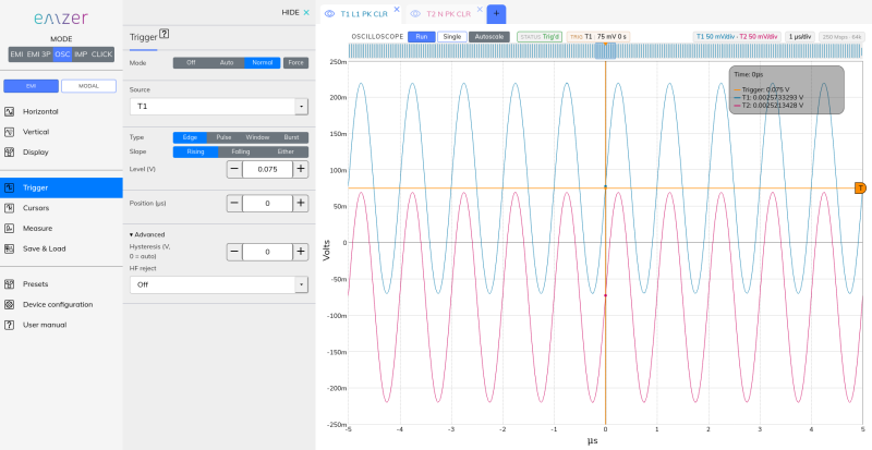
Figure 18. Trigger menu.
The red cursors on the graph show the trigger level and the trigger position. Both can be dragged with the mouse or typed in the Trigger menu (Figure 19).
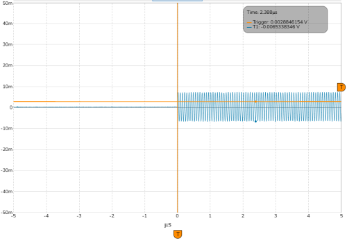
Figure 19. Data capture using the trigger option.
The trigger watches every sample at the full 250 Msps, whatever the time division factor: a glitch of a few nanoseconds triggers also at slow time divisions, widths and times are set to 4 ns at any setting, and the trigger point is placed at the exact sample where the condition was met.
5.10.1 Mode
- Normal: a capture is only shown when the trigger condition is met. If the condition never occurs, the screen keeps the last capture. This is the mode to capture rare events.
- Auto: if the trigger condition does not occur within 100 ms, a capture is taken anyway, so that a signal is always visible. Use it to find a signal before setting the level.
5.10.2 Source
The trace whose channel triggers the capture, chosen with the trace buttons (one per trace, in its colour; the selected one is filled). The same buttons are used in the clickmeter trigger. EXT (the external trigger input) is listed but disabled: the input is not available on the connectors of this instrument.
- Off: the trigger is not used; captures are taken freely, without synchronising to the signal. With the trigger off, the rest of the trigger settings are shown dimmed: they can still be set, and apply when the trigger is switched on.
- Trace: the trigger is taken from the analog channel of the trace selected in Source.
5.10.3 Type
- Edge: the trigger fires when the signal crosses Level in the direction set by Slope: Rising, Falling or Either.
- Pulse: the trigger fires on a pulse whose width is narrower or wider than Width (µs), as selected in Condition. A pulse starts and ends when the signal crosses Level. Slope selects the polarity: Positive (a pulse above the level) or Negative (a pulse below the level). With “Narrower than” the trigger point is the end of the pulse, because its width is only known then. With “Wider than” the trigger point is the instant the pulse exceeds Width, while it is still in progress. Widths from 4 ns to about 17 s can be set.
- Note on long pulses: the oscilloscope uses the receiver input, which has a 9 kHz high-pass filter (time constant about 18 µs). A pulse longer than about 20 µs does not stay above the level: it reaches the input as two short spikes, one at each edge. “Wider than” is therefore only useful for widths up to a few tens of microseconds. To pick out events separated by a long time (milliseconds or more), use Burst with Idle set to the quiet time before the event.
- Window: the trigger fires when the signal enters or leaves the band between Level and Level 2, as selected in Condition (Entering / Leaving). The two levels can be given in either order. With hysteresis, the signal must first be that far outside the band before entering it counts, and that far beyond an edge before leaving counts.
- Burst: an edge, as with Edge, that only fires when the signal has stayed without crossing the level for at least Idle (µs) before it. It triggers on the first edge of each burst of pulses or oscillations, and not on the edges inside the burst. With an Idle of 0 it is the same as Edge.
5.10.4 Level, position and advanced settings
- Level (V): voltage that the signal must cross.
- Position (µs): position of the trigger point on the time axis. At 0 µs the trigger point is at the centre of the screen, so the same amount of signal is shown before and after it. A positive offset moves the trigger point to the right and shows more of the signal before the trigger.
- Advanced → Hysteresis (V): a crossing is only accepted after the signal has first moved this amount away from the level on the other side. For a rising edge, the signal must go below (Level − Hysteresis) before a crossing up through Level fires. It prevents noise around the level from triggering repeatedly, or on the opposite edge. 0 is automatic: a tenth of a division of the trigger trace, more on the most sensitive ranges (5 mV/div and below), where the input noise is larger. Set a value when the signal is smaller than about a quarter of a division (a smaller hysteresis) or very noisy (a larger one): a signal that does not go beyond the hysteresis never arms the trigger.
- Advanced → HF reject: a low-pass filter in front of the trigger only, with its corner at 5 MHz, 620 kHz or 78 kHz. The trigger then follows the slower part of the signal, and ringing or noise above the corner does not fire it: for instance, to trigger on the switching frequency of a power converter without the ringing of each transition triggering again. The trace and the capture are not filtered. As in any filter, the trigger point is delayed, by about 1/(2π × corner): 32 ns at 5 MHz, 0.26 µs at 620 kHz, 2 µs at 78 kHz.
5.10.5 Force
The Force button triggers the capture immediately, whether or not the trigger condition occurs. It is useful in Normal mode to check the signal when the trigger never fires. It is only available with the trigger on.
5.10.6 Trigger status
The status of the trigger is shown next to the scale information at the top right corner of the graph:
| Status | Meaning |
|---|---|
| Ready (yellow) | The oscilloscope is waiting for the trigger condition. |
| Trig'd (green) | The last capture was started by the trigger condition (or by Force). |
| Auto (blue) | The last capture was taken in Auto mode because no trigger occurred within 100 ms. |
| Stop (red) | The acquisition is stopped, or a Single capture has been completed. |
When a setting does not fit the hardware (a trigger level beyond the input range, a width or idle time beyond its limit), it is brought to its limit, the menu shows the value in force, and a notice says what changed. When a capture fails or is incomplete (for instance samples lost by a converter), a red notice is shown over the graph: the trace on the screen may then not be current.
5.11 Run / Stop / Single
The Run / Stop and Single buttons, in the bar above the graph next to the trigger status, control the acquisition:
- Run / Stop: starts the continuous acquisition, or stops it and freezes the last capture on the screen.
- Single: takes one capture and stops. With the trigger on, it waits for the trigger condition, which makes it the usual way to capture a single event: set the trigger in Normal mode, press Single, and the event remains on the screen when it occurs.
5.12 Cursors
Cursors allow the user to manually identify points on a scope trace. In the Cursors menu, two time cursors (vertical lines) and two amplitude cursors (horizontal lines) can be switched on, dragged on the graph or typed. The time cursors move from one sample of the capture to the next. Under the graph, the value of each cursor is shown and, with both cursors of a pair on, their difference, cursor 2 minus cursor 1: ΔX and 1/ΔX for the time cursors, ΔY for the amplitude cursors. The amplitude cursors are in the volts of the active tab.
The time cursors also delimit the automatic measurements when their range is Cursors (see Measurements).

Figure 20. Cursors option.
5.13 Measurements
The Measure menu adds automatic measurements of the traces, shown live in a table under the graph (Figure 21). Choose the measurement and the trace it is taken on (Source), and press Add measurement. Up to six measurements can be shown at once; each one is removed with its × button.
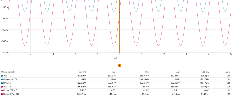
Figure 21. Measurements table.
The measurements are computed on the samples of the capture, not on the points drawn on the screen, so they are exact also with deep memories. Range selects which samples:
- Screen: the part of the capture shown on the screen (it follows the zoom).
- Whole capture: the whole capture, including the part off the screen.
- Cursors: the samples between the two time cursors, which are switched on if they are off. With one of them off, the measurements are empty.
| Measurement | Definition |
|---|---|
| Vpp | Maximum minus minimum. |
| Max / Min | Highest and lowest sample. |
| Top / Base | The flat high and low levels of the signal: the most frequent levels of the upper and lower half of the histogram of the samples. When the signal has no flat levels (a sine, a triangle), Max and Min. |
| Amplitude | Top minus Base. |
| Mean | Average of the samples (DC value). |
| RMS | Root mean square of the samples, DC included. |
| AC RMS | RMS with the mean removed (standard deviation). |
| Frequency / Period | From the spacing of the rising edges, averaged over all the periods in the range. |
| +Duty | +Width divided by the period, in %. |
| +Width / −Width | Time from a rising to the next falling edge, and from a falling to the next rising edge, averaged. |
| Rise time / Fall time | Time between 10 % and 90 % of the amplitude (Base to Top) on the rising and falling edges, averaged. |
| Phase | Phase of the trace against a second trace chosen in Against, at the fundamental frequency of the second one, from −180° to 180°. Positive when the trace lags. |
| Delay | The same, as a time: the phase divided by 360° and by the frequency, within half a period. Positive when the trace lags. |
Edges are taken at 50 % of the amplitude with a hysteresis that adapts to the noise of the signal (three times the noise, at least ±10 % of the amplitude), so noise around the middle level does not count as an edge; a period that differs from the others by more than 25 % is left out. Timing measurements use up to the first 1000 edges of the range. A measurement that cannot be made (a flat signal, less than one period in the range) is shown as —.
Phase and Delay compare two traces of the same capture: choose Phase or Delay in the Between traces group, the trace to measure in Source and the reference in Against. Both traces are compared at the fundamental frequency of the reference, over a whole number of its periods in the range, which averages every period and makes them insensitive to noise: on a clean signal they resolve hundredths of a degree and a few picoseconds. They are also the way to measure the delay between the inputs, or through a cable or a probe.
In Peak detect, Vpp, Max and Min are taken from the minimum/maximum pairs, and the other measurements from the middle of each pair. When the windows are too long for the signal (few points per period), the timing measurements are shown as — rather than a false value: use a faster time division factor, a deeper memory or the Normal acquisition.
Important! A rise or fall time shorter than two samples is set by the sampling frequency, not by the signal: it is shown as “< value”. Increase the memory depth or reduce the time division factor to measure it.
Statistics. For each measurement the table shows the current value and, over the captures since the statistics were last cleared, the mean, minimum, maximum, standard deviation and number of values. Each capture is counted once, also when the screen is redrawn while stopped. The statistics are cleared with Clear statistics, and also when the time division factor, memory depth, acquisition, amplitude division factor, trigger level or offset, the channel of the trace, or the range (or the cursors that delimit it) change.
Important! With deep memories (1M samples and more) the measurements take time on the instrument: up to a few seconds for all the timing measurements on a 10M capture. Use the Screen or Cursors range, or fewer measurements, for a faster update.
5.14 Saving the capture
In the oscilloscope mode, the Save menu saves the capture itself rather than the points drawn on the screen (which, with deep memories, are minimum/maximum pairs), so Save measures in CSV is not offered. To save every sample of the last capture of the traces shown, choose the format next to Capture in the Save menu and press Save full capture. The file is named after the date and time the capture was taken (for instance emscope_capture_20261023_101112).
- CSV: one row per sample, with the time in seconds from the trigger and the voltage of each trace. The settings of the capture come first, as lines starting with #. It opens in spreadsheet editors. Available up to 1M samples (about 35 MB for two traces); the conversion is done by the web browser and takes a few seconds.
- Binary: every sample of any capture, up to 10M, in a compact file (2 bytes per sample and trace, 80 MB for 10M samples of four traces). It is read with a script.
The binary file starts with a text header (key=value lines) of the size given by header_bytes (2048 bytes; 1024 in files saved by earlier versions), followed by the samples as 16-bit signed little-endian integers, the traces interleaved (sample 0 of every trace, then sample 1, and so on). The header holds:
- samples, traces, names, sample_rate_hz, trigger_sample, and volts_per_count and units, one value per trace in the order of names. The time of sample i is (i − trigger_sample) / sample_rate_hz, and the value is count × the volts_per_count of its trace, in its unit (V, or V^2 for a product).
- The settings the capture was taken with: capture_time_utc, instrument (product and serial number), acquisition and combine, time_per_div_s, and per trace volts_per_div, vertical_offset_v and horizontal_offset_s; and the trigger (trigger, and when it is on trigger_mode, trigger_source, trigger_type, trigger_slope, trigger_hf_reject, trigger_position_s, trigger_level_v, trigger_hysteresis_v, and the level 2, condition, width or idle time of its type).
An Average capture is saved to the nearest count. An Envelope or a Peak detect capture is saved as its minimum/maximum pairs: two values per window, the minimum first, at twice the sampling frequency.
Ready-made readers for Python and MATLAB: read_emscope_capture.zip. Each one is a function that returns the time of every sample (in seconds, 0 at the trigger), the value of every trace in its unit, and the names and units of the traces:
- Python (needs numpy):
t, values, names, units = read_emscope_capture(“emscope_capture.bin”). Run as a script,python read_emscope_capture.py emscope_capture.binprints a summary of the file. - MATLAB:
[t, values, names, units] = read_emscope_capture(“emscope_capture.bin”);
Both also read the files saved by earlier versions, which have one volts_per_count for all the traces.
6. Clickmeter Operating Instructions
This section introduces the clickmeter mode and explains its main utilities. The clickmeter mode is activated when clicking on the CLICK button.

Figure 22. Clickmeter button.
6.1 Introduction
The EMSCOPE Clickmeter mode is accessed via a web browser, as previously described. Upon the first connection—or when using the “Start with default settings” option—the system automatically launches a measurement using the default configuration. This includes a single trace measuring the four Line channels, a Result Table below, and the configuration menu, as illustrated in Figures 23 and 24. The menus follow the order of a test: Test setup, Input (reference level and losses, as the Amplitude menu of the EMI mode) and Channels, then Report and Save & Load; the Start, Pause, Stop and Reprocess buttons are under User manual, with the elapsed and remaining time of the test below them.
The four Line channels correspond to the following frequencies: 150 kHz (Channel 1), 500 kHz (Channel 2), 1.4 MHz (Channel 3), and 30 MHz (Channel 4).

Figure 23. Web app interface.

Figure 24. Table results.
The most relevant information regarding the measurement for each trace is provided in the trace tab.
If the user modifies the measurement configuration and closes the session, the next time the user connects again to the EMSCOPE, the last configuration before closing is recovered.
Next Sections relate important considerations for the measurements and describe the relevant settings of the function keys.
6.2 Test Setup
The Test setup menu (Figure 25) holds everything that defines the test, in the order it is prepared: the configuration mode, the limit the test is judged against, the test duration and the measurement type. The bar above the chart summarises the configuration in force (RBW, reference level, losses, configuration, limit, measurement type, duration and recorded channels, and the result once there is one); clicking an item opens its menu. A missing limit is shown in red.

Figure 25. Test setup menu.
Configuration Mode
The Configuration mode dropdown selects the configuration applied to the clickmeter test. It contains the following entries:
- Default: the configuration the instrument starts with.
- Custom: selected automatically as soon as any setting is edited by hand, so that the dropdown never shows a configuration that is no longer applied.
- Equipment under test: a catalogue of equipment from CISPR 14-1 Annex A, grouped by its sections (A.1 Motor operated equipment for household and similar purposes, A.2 Electric tools, etc.). Selecting an equipment applies its configuration (click rate mode, factor f, programme mode, time limit) and selects its limit, so that the test can be started straight away. The line under the dropdown shows the clause of CISPR 14-1 that describes the operating conditions of the equipment, and the limit applied. For some equipment the limit is not set and must be chosen in Limit. If the limit is not available in the instrument, the rest of the configuration is applied and a message asks to select the limit by hand.
- Saved configurations: the configurations saved by the user.
The Save as device config button saves the current settings, including the selected limit, under a name. The Delete config button deletes the selected saved configuration. Configurations saved with earlier versions do not include the limit; when they are applied, the limit is left unchanged.
If the limit is changed by hand while an equipment that prescribes a limit is selected, the configuration switches to Custom.
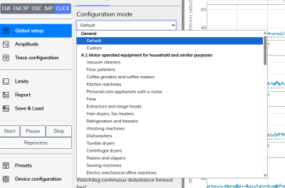
Figure 26. Configuration mode dropdown with the equipment catalogue.
6.2.1 Limit
Limit selects the standard limit the test is judged against, with the Activate standard option. Only limits corresponding to Band B are available in this mode. The limit can also be selected automatically by choosing an equipment in the Configuration mode; selecting by hand a limit different from the one of the selected equipment switches the configuration to Custom.
Manage limits opens the management of the limits, as in the Limits menu of the EMI mode: Create, Edit and Delete a limit, Load from file and Save to file, and Reset to factory to restore the limits supplied with the instrument (Figure 27).
Figure 27. Limit and limit management in the Test setup menu.
Important! A standard limit must be selected and the “Activate standard” option must be enabled before a test can be started.
The limit cannot be changed while a test is running or paused, or while a measurement is being reprocessed.
6.2.2 Test Duration
Time limit sets the test duration (hours:minutes:seconds). It must always be less than or equal to the maximum shown next to it (in parentheses), which depends on the number of recorded channels (see Channels) and includes the space taken by the measurement currently stored, since it is deleted when the next test starts. The test duration can be changed while the test runs.

Figure 28. Test duration.
6.2.3 Click limit

Figure 29. Click limit box.
If selected (as shown in Figure 29), the test stops when the number of measured clicks reaches the value specified by the user. If not selected, a default click limit of 40 clicks is applied.
6.2.4 Mode Programme
If the Equipment Under Test (EUT) operates according to a defined programme, the Programme option must be selected. In this mode, the following conditions must be preserved:
- If the click rate observed during a complete programme is less than or equal to 0.5 clicks per minute, and the programme duration exceeds 20 minutes, the minimum observation time is equal to the duration of a complete programme.
- Otherwise, the minimum observation time is either:
- The total duration of the minimum number of complete programmes required to detect 40 clicks at one of the two reference frequencies, or
- The total duration of the minimum number of complete programmes that exceeds 120 minutes, if after 120 minutes fewer than 40 clicks have been recorded.
6.2.5 Watchdog continuous disturbance timeout
The longest time, in milliseconds, a disturbance may stay above the limit and still be analysed as a click (600 ms by default and at minimum). A disturbance that lasts longer is a continuous disturbance, not a click: the test fails and stops.
6.2.6 Measure Clicks/Manual Click Rate/Switching Operations
The Measurement type offers three operating modes:
- Measure Clicks (default mode): The test continues until 40 clicks are detected or until the user-defined measurement time is reached.
- Manual Click Rate: Allows the user to manually set the click rate (Nc, clicks per minute) in Rate.
- Switching Operations: In this mode, a new click rate (Ns) is computed from the number of Operations and the Factor of the type of EUT, according to Annex B (Table B.1) of CISPR 14-1.
6.3 Channels
The Channels menu can be seen in Figure 30.

Figure 30. Channels menu.
6.3.1 Recorded Channels
Recorded channels selects which channels the test stores: Line (L), Neutral (N), Common Mode (CM) and/or Differential Mode (DM). The number of recorded channels directly affects the maximum test duration (see Test Duration). The recorded channels cannot be changed while a test is running.
6.3.2 Measure Channel
Shown in selects the channel shown in the selected tab: L-G, N-G, CM or DM.
6.3.3 Margin Peak Detectors
There are four text boxes, one per measuring frequency: CH1 (150 kHz), CH2 (500 kHz), CH3 (1.4 MHz) and CH4 (30 MHz). The margin value is used to shift the standard limit line upward in those cases where the measured noise exceeds the specified limit.
The margin decides which disturbances are counted as clicks, so it cannot be changed while a test is running or paused, or while a measurement is being reprocessed.
6.4 Report
The Generate Report button creates an automatic test report in a new web browser window. If desired, the report can be downloaded as a PDF by clicking the Download button (as shown in Figure 31). Figure 32 shows an example of a result table shown in the report's window.

Figure 31. Report (download button).

Figure 32. Report's table.
The report always covers the whole measurement, regardless of the zoom applied to the chart. It describes the measurement as it was analysed: the limit in the title, the limit values, the margins and the click rate mode are those used in the analysis, even if the controls have been changed afterwards. A finished measurement can therefore be reported even after the limit has been deactivated.
The report includes:
- Correction factors: the loss tables applied to the measurement when it was recorded: the name of the external loss table and/or “Internal LISN”, or “None” when no correction was applied. A measurement recorded with an earlier version shows “Unknown (not recorded)”. If the correction factors selected now are different, a message warns that the report describes the measurement as it was recorded, and that the measurement must be reprocessed to apply the new ones (see Reprocess).
- Overload marks: the time intervals affected by ADC saturation are drawn as light red bands on the plot, and the instants where the ADC actually clipped as dark red marks at the top of the plot (see Overload below).
- Detected clicks: after the decision flowcharts, one zoomed graph centred on each detected click, grouped by channel, two clicks per page in the PDF. Under each graph: click number, time, duration and duration class, peak (Pk) and quasi-peak (QPk) levels, limit L and relaxed limit Lq, and the exception applied, if any. Up to 40 clicks are detailed per channel; when a channel has more, a note under its last graph says “Only the first N clicks of this channel are detailed”.
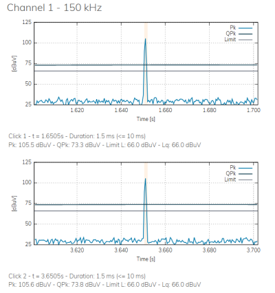
Figure 33. Zoomed graph of detected clicks in the report.
6.5 Start/Pause/Stop
These buttons are under User manual in the main menu, with the elapsed and remaining time of the test below them (Figure 34).

Figure 34. Start, Pause and Stop options.
- Start: Initiates the clickmeter test, after a window that shows the whole configuration to review and confirm. Starting a new test deletes the measurement previously stored. It is only available when a limit is active.
- Pause: Temporarily pauses the clickmeter test. The test can later be resumed by clicking the Start button or terminated by clicking the Stop button.
- Stop: Terminates the clickmeter test.
The click analysis needs a continuous observation of the signal. If part of the signal cannot be acquired (the hardware buffer overflows, or a data transfer from the hardware does not complete), the instrument stops the test by itself and shows a message starting with “Test stopped:” that gives the reason. The results up to that moment are kept, and the recorded data can be reprocessed (see Reprocess), but the test is not continuous and should be repeated for a compliance decision.
A test is analysed from beginning to end with a single set of settings. Therefore, while a test is running or paused, the following settings cannot be changed: Configuration mode, limit, click rate mode, timeout of continuous disturbance, test duration, margin peak detectors, Reference Level, and external and internal losses. Trying to change them shows the message “Settings locked” and the field returns to the value in force. Stop the test to change them.
The recorded measurement is kept when the server restarts or the instrument is switched off, until the next test starts (it is deleted on the first start after a software update). When the clickmeter mode is entered again, the measurement is recovered with its chart, results table and report, and a message indicates when it was taken (“Measurement recovered from …”). Reading back a long measurement takes some time (around three and a half minutes for two hours of recording); the progress is shown at the top of the page.
6.6 Reprocess
The Reprocess button, below the Start/Pause/Stop buttons, re-analyses the whole recorded measurement with the limit and the settings in force now, without repeating the test. It is useful when a setting (for instance, the limit, the click rate mode or the number of switching operations) or a loss table has to be corrected after the test, without operating the EUT again.
The button is available only when the test is stopped, a limit is active and there is a recorded measurement. The whole measurement is always re-analysed: zooming the chart does not change what is analysed.
While a measurement is being reprocessed:
- The progress is shown at the top of the page (“Reprocessing the recorded measurement, please wait… N %”), and the results table is updated as the re-analysis advances.
- The Start, Pause and Stop buttons are disabled, and the settings cannot be changed (message “Settings locked”).
At the end, the message “The recorded measurement has been re-analysed.” is shown and the chart is refreshed. If it cannot be completed, a message asks to check that the test is stopped and that there is recorded data.
Change of losses. The stored measurement keeps the amplitudes it was recorded with. When the external losses or the internal LISN losses are changed after the test, a message indicates which correction changed and by how much (for instance “the external losses (by 10.00 dB) changed since this measurement was analysed, so its results no longer apply. Re-analyse it to update the table.”). Pressing Reprocess then asks for confirmation, with an estimate of the time needed (“Reprocessing it takes about … and the instrument cannot measure meanwhile.”). If accepted, the stored measurement is first converted to the new losses and then re-analysed; if cancelled, the measurement keeps the calibration it was taken with. Measurements recorded with an earlier version are re-analysed as they are, without conversion.
Figure 35. Reprocess button.
6.7 Overload
When the ADC saturates during a clickmeter test, the affected time intervals are marked on the chart:
- A light red band covers the interval where the measurement is not valid: the saturation itself plus 0.8 s during which the quasi-peak reading recovers from it.
- A dark red mark at the top of the chart shows the instants where the ADC actually clipped.
The label OVERLOAD DETECTED is shown under the chart while the measurement contains any saturation. The same marks are drawn in the report. To avoid overload, raise the Reference Level before starting the test (see Reference Level in the EMI section) or use an external attenuator.
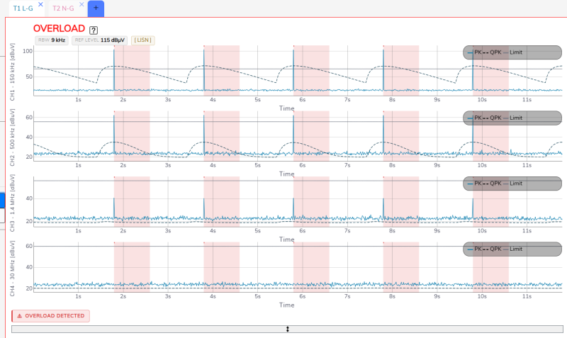
Figure 36. Overload marks on the clickmeter chart.
7. Applications
7.1 Conducted Emissions
All electric and electronic devices are potential generators of EMI. The term EMI thus refers to the unintended electromagnetic energy emitted by a device which propagates itself along cables or through the air and couples with other devices that are present in the surroundings. These electromagnetic fields (conducted or radiated interference) may generate interfering currents and voltages into nearby equipment and therefore can cause possible malfunctions. In order to prevent and control such interference there are a number of national and international standards, like IEC, which specifies limits and methods of tests. Moreover, within the European Union the application of several European Norms on Electromagnetic Compatibility is enforced by law and therefore the commercialization and use of all the electric and electronic equipment is subject to the measurement of the EMC characteristics, which must be within well-defined limits.
The conducted emissions are the noise currents and voltages that propagate through the power cord or harness to other components/systems or power grid. The EMI currents (or voltages) of the two conductors relative to each other and with reference to the ground form a vector system where two kinds of currents (or voltages) are present. They are:
- The differential-mode noise (DM), defined as the noise that appears across power supply lines and is in series with the power supply line, and the noise current flows in the same direction as the power supply current (Figure 37.a).
- The common-mode noise (CM), defined as the noise current that has leaked via a stray capacitance through ground and returns to the power supply line (Figure 37.b).
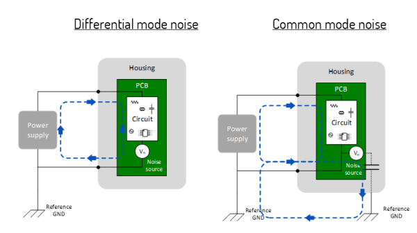
Figure 37. Modal definition of interference: (a) DM. (b) CM.
To reduce the conducted emissions a power-line filter needs to be placed between the power-line terminals and the Equipment Under Test (EUT). In its simplest structure, it contains an X capacitor between line and neutral to mitigate the DM, and a common-mode choke (CMC) and two Y capacitors from line to ground and neutral to ground to mitigate the CM.

Figure 38. Power-line filter components.
Therefore, since these filter components only have effect on one of the modal components (either CM or DM), it is important to measure the modal interference components in order to build a suitable power-line filter. Thanks to the simultaneous measurement of the line and neutral terminals, EMSCOPE is able to recover and provide the measurements of the modal emissions.
7.2 Measurements According to Standards
The design philosophy behind EMSCOPE prioritizes innovation, compliance with relevant standards, and user-friendly reliability. This ensures that EMSCOPE serves as a foundational building block for any conducted emissions system, enabling the measurement and evaluation of electric or electronic devices throughout their lifecycle—from initial design stages to final certification.
The demand for precise measurement of conducted EMI noise compels equipment manufacturers to rely on dependable tools to verify compliance with applicable standards and regulations. EMSCOPE emerges as the ideal solution, offering seamless usability from prototype debugging to final certification. It delivers exceptional performance in line with industry standards while maintaining a compact, lightweight, and user-friendly design.
Its intuitive web-browser interface allows for immediate operation without requiring extensive training or specialized knowledge, enabling users to focus entirely on analyzing measurement results.
For accurate assessments, the EUT must be installed in accordance with the manufacturer’s instructions, ensuring adherence to standard operating conditions.
7.3 Measuring the EMI Voltage
ElectroMagnetic Interference (EMI) voltage measurements on power supply lines or on signal lines are carried out by means of “Coupling Networks” (e.g. LISNs) or other transducers (e.g. voltage probes). The frequency range is dictated by the applicable standard, which goes from 9 kHz to 30 MHz in most commercial applications.
7.3.1 Measuring principle with a LISN
Important! Before using the LISN follow the provided Safety information. Not following it can result in important damages, serious injuries and death.
Any LISN has three main objectives:
- To present a constant impedance to the power input of the EUT, in order to get repeatable measurements of the EUT noise present at the LISN measurement port.
- To prevent the high-frequency noise of the power source from coupling in the system. A LISN functions as a low pass filter, which provides high impedance to the outside RF noise while allowing the low-frequency power to flow through to the EUT.
- To couple the high frequency noise signal emitted by the EUT to the input of the measuring equipment (EMSCOPE receivers).
The LISN from EMSCOPE has been designed under the CISPR 16-1-2 standard for evaluating and characterizing the operation of the EUT. It is a V-type Network with an impedance of 50 Ω/50 μH + 5 Ω. The schematic of this LISN can be seen in Figure 39. It includes additional capacitors and inductors for filtering and has an operating frequency range of 9kHz to 30MHz.

Figure 39. Schematic of the EMSCOPE’s LISN.
7.3.2 Test Setup according to CISPR 16-2-1
Figure 40 shows an example of the test setup for RFI voltage measurement according to CISPR 16-2-1. The EUT is placed on the top of a table at 0.8 m from a horizontal earthed conducting surface, and at 0.4 m from a vertical earthed conducting surface.
The LISN shall be bonded to the reference conducting surface.
A floor-standing EUT is placed 0.1 m above a horizontal earthed conducting surface of at least 2 m x 2 m in size. This surface shall exceed by at least 0.5 m the projection of the EUT on the conducting surface.
The power cable should be 1 m long; longer cable should be centrally bundled for at least 40 cm.
EUTs without a PE (Protective Earth) conductor and manually operated EUTs shall be measured in conjunction with an auxiliary screen or an “Artificial Hand”, as duly specified in the relevant standards.
All the details and information on the test setup are given in the latest version of the applicable Standard.

Figure 40. Test setup for RFI voltage measurement.
7.3.3 Guidance on a preliminary Measuring Procedure for Band B
A step-by-step example of a conducted test manually performed is the following:
- Switch ON the EMSCOPE and connect to it as described above.
- Introduce a Reference Level between 110 and 125 dBµV and a RBW of 9 kHz selecting the proper frequency measurement range in the Frequency/Sweep menu. Adjust the Scale/Div to 10 dB.
- Set the Input attenuator to Automatic mode.
- Introduce a Span between 150 kHz and 30 MHz (check the Common values option).
- Set the dwell time to 2 seconds.
- Open as many traces as detectors desired and select the suitable one in each of them (for instance, peak and average detectors).
- Select L-G or N-G measurement in each trace (if both are desired, do it in different tabs).
- Go to the Limits tab and find the desired standard. If it doesn’t exist, create a new one. Then activate it to see the limits in the measurement plot.
- Connect the two outputs of the LISN to the two RF inputs of the EMI receiver using the N bridges.
- With the EUT switched OFF, check that the ambient RF disturbances are at least 20 dB below the desired limit of emissions. If the ambient noises are low enough continue to the next step, otherwise take all the necessary steps to reduce the ambient disturbances (e.g. go to a shielded room).
- Switch ON the EUT and wait for the measurement (the measurement time is equal to the dwell time, in this case, two seconds).
- Adjust the Dynamic Range and the Reference Level to the most convenient visualization.
- If the results are satisfactory, go to the Report tab and press the button List of maximum emissions to list the critical emissions.
- Press the button Generate Report to obtain an automatic report of the measurements.
7.3.4 Remarks and Hints for Measuring
To avoid errors caused by ambient interference, measurements should be carried out inside a properly shielded room. Different sites, like basements or other rooms with low ambient interference, are often enough for a preliminary evaluation.
Conducted measurements do not strictly require any anechoic environment.
8. Updating Firmware and Software
To update the firmware, access the main interface, go to “Device configuration” and click on “Update Device”; alternatively, type the following address in the URL field:
http://emscope-xxxx.local/update.html
where xxxx are the last 4 characters from the SN of your EMSCOPE. The SN is provided in the rear panel. A web interface similar to that shown in Figure 41 appears.
If EMSCOPE has access to https://emzer.com/, the user will be notified and prompted to update the device automatically once the user authorizes it.
If the EMSCOPE can’t reach the Internet, the user can manually download the latest firmware image from https://emzer.com/updates and upload it to the EMSCOPE by clicking on the “manual update” link and selecting the update file with the “Choose File” button.

Figure 41. Web interface for an image updating.
9. Remote control
The EMSCOPE software consists of a WebSocket server listening on port 8010 of the machine, and a web server listening on the standard http port 80 that serves the frontend html and related files.
For users that want to write an application for automatic configuration and measurements, EMZER provides the WebSocket API specification (PDF), and a Javascript API that includes an implementation and example.
10. Maintenance
Maintenance of the equipment is limited to external components such as cables.
During operation, inside the equipment there are DANGEROUS voltages that could be contacted. To prevent electrical shock, do not open the equipment.
Clean the exterior of the equipment using a damp cloth and mild cleaner. Always unplug the unit before cleaning.
Product may be opened only by authorized, specially trained personnel. Before performing any work on the unit, it must be disconnected from the mains. Only technical personnel authorized by EMZER can perform any adjustments, replacement of parts or repair.
11. Disposal
This equipment is designed and manufactured with materials and components that can be recycled minimizing the environmental footprint.
A product that is labeled with a crossed-out wheeled bin symbol means it is covered by the European Directive 2012/19/EU and cannot be disposed of in normal household waste at the end of its life.

Figure 42. Label according to EU WEEE directive.
Please act according to your local rules. The correct disposal of your old products will help prevent potential negative consequences for the environment and human health.
12. Troubleshooting Guide
Measurement hardware and ADC calibration messages
- Measurement hardware: The measurement hardware did not start (R5 firmware initialisation failed): no measurement is possible. The instrument could not start its measurement processor after loading a mode, so no measurement is shown. Restart the instrument, and contact service if the message persists.
- ADC calibration: The ADC inputs could not be calibrated (…) and run on their default timing. The measurements may be degraded. Restart the instrument, and contact service if the message persists.
Problems with MDNS
To make the connection to the EMSCOPE devices as easy as possible, the protocol MDNS is used. Thanks to it, the user only needs to type the following address in the URL field for the connection:
http://emscope-xxxx.local/
where xxxx are the last 4 characters from the SN of the EMSCOPE.
In some specific scenarios, the MDNS can fail, obtaining something similar to:
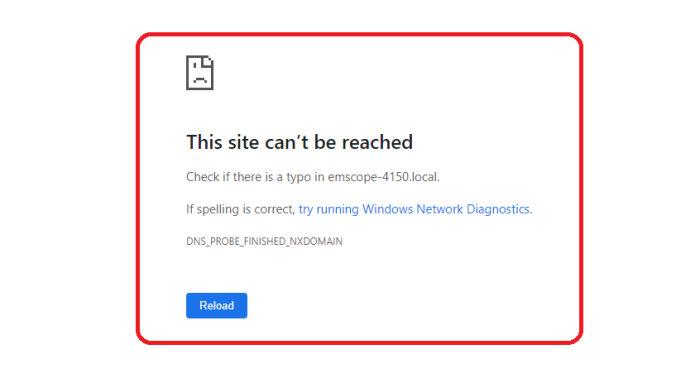
Figure 43. Web text shown when EMSCOPE is not reached.
There are multiple reasons for this behavior. To overcome this problem, please, follow the steps below:
- Check that your EMSCOPE is properly connected. The SFP Multi-mode optical fiber must be connected between the EMSCOPE's SFP connector (rear panel of the device) and the fiber to Ethernet/USB converter. The converter must be connected to a LAN or directly to the PC.
- Check that your EMSCOPE is switched on. The startup lasts approximately one minute. Once it has finished, the leftmost LED is fixed green, the center LED is flashing yellow, and the rightmost LED is fixed green as well.
If the EMSCOPE is properly connected and switched on, but it cannot be reached yet, try the following steps:
- Keeping the EMSCOPE switched on, restart the PC. Windows usually only updates the MDNS table when it starts. After restarting the PC, try to connect to the EMSCOPE using the MDNS address.
- If the previous step does not solve the connection problems, try connecting to the EMSCOPE using its IP address. For instance: http://10.30.0.171/
- If the IP address is not known, install the Bonjour software. With this software, it is possible to check if the EMSCOPE’s web service is available and, if so, which IP address it has. Then, try to connect directly using the IP address (previous step).
Having a LAN with a proxy server can be a reason to reach the EMSCOPE when using the IP but not when using the MDNS address. To overcome this problem, please read the following Section.
How to Bypass Proxy Server for Local Addresses in Windows 10
In case of using Windows 10 connected to a LAN with a proxy server, the MDNS will not work (only works directly writing the IP address of the EMSCOPE in the web browser). Windows does not exclude the local website addresses like intranet or localhost from proxy by default. To bypass the proxy, follow the steps of one of the options below:
Using Internet Options
- Press “Win + E” shortcut keys to open File Explorer.
- Type “control panel” in the address bar and press enter key to open Control Panel app.
- Change the “View by” option to “Category” to view the details.
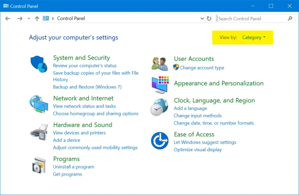
Figure 44. Control Panel Category View.
- Click on “Network and Internet” option and then click on “Internet Options”.
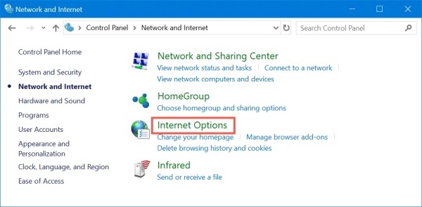
Figure 45. Open Internet Options from Control Panel.
- Alternatively, you can use Windows Search box to search “internet options” and open the Internet Properties dialog box.
Figure 46. LAN Settings in Windows 10.
- Go to “Connections” tab and click on “LAN settings” button. This will open “Local Area Network (LAN) Settings” pop-up. Enable “Use a proxy server for your LAN” check box to enter the IP address and port of your proxy server.
Figure 47. Setup Proxy Server in Windows 10.
- A proxy server is now set up and all the traffic of the computer goes through it. For providing exception or bypassing your local intranet website addresses, enable “Bypass proxy server for local addresses” check box and click on “Advanced” button.
Figure 48. Provide Exceptions in Proxy.
- Under “Exceptions” box, type all the website addresses you do not want to use proxy. Use semicolon to separate each address you want to exclude. Click “OK” to apply your changes. In this case: http://emscope-xxxx.local/, or just “emscope-xxxx”.
Using Settings App
- Press “Win + I” keys to open the Windows Settings app and go to “Network & Internet” section.
- Go to “Proxy” section and enable “Use a proxy server” option under “Manual proxy setup” section.
Figure 49. Manual Proxy Server Setup.
- Type the addresses in the text box to exclude them from proxy access. In this case: http://emscope-xxxx.local/, or just “emscope”.
- Enable the checkbox “Don’t use the proxy server for local (intranet) addresses” option.
- Click “Save” button to save your changes.
Using Firefox Network Settings
All the browsers like Chrome, Edge and IE use the computer’s network settings for proxy. However, Firefox has standalone browser settings that allow you to add proxy and exceptions within the browser. Remember, this method is effective only within Firefox browser and your computer’s network will still follow the default settings from Internet Options.
- Go to “about:preferences” page, scroll down to “Network Settings” and click on the “Settings…” button.
Figure 50. Firefox Network Settings.
- This will open “Connection Settings” pop-up within Firefox.
- Choose either manual or automatic proxy configuration option.
Figure 51. Setup Proxy in Mozilla Firefox.
- Type the exception for local and other website addresses under “No proxy for” text box. In this case: http://emscope-xxxx.local/, or just “emscope”.
- Click “OK” to save your changes.
Return for Repair form
Dear Customer,
Thank you for purchasing an EMZER’s product. You now own a high-quality instrument that will give you many years of reliable service. EMZER recognizes the importance of the Customer as reason of existence; in this view, any comment and suggestion you would like to submit to the attention of our service organization is kept in great consideration. Moreover, we are continuously improving our quality, but we know this is a never-ending process. We would be glad if our present efforts are pleasing you. Should one of your pieces of EMZER equipment need servicing you can help us serve you more effectively by filling out this card and enclosing it with the product. Nevertheless, even this product will eventually become obsolete. When that time comes, please remember that electronic equipment must be disposed of in accordance with local regulations. This product conforms to the WEEE Directive of the European Union (2012/19/EU) and belongs to Category 9 (Monitoring and Control Instruments). You can return the instrument to us free of charge for proper environment friendly disposal. You can obtain further information from your local EMZER Sales Partner or by visiting our website at www.emzer.com.
Service needed
- Calibration only
- Repair
- Repair & Calibration
- Certified Calibration
- Other
Company:
Address:
Technical contact person:
Phone number:
Equipment Model:
Serial Number:
Accessories returned with unit:
- None
- Cable(s)
- Power cable
- Other:
Observed symptoms/problems: